|
Objective:
Learn how to do LSRTM using the visco-acoustic wave-equation. The adjoint and linear modeling operators are based on standard migration and de-migration operators.
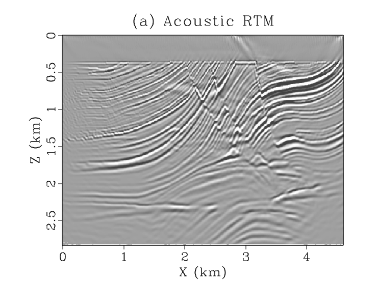
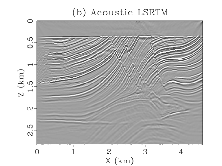
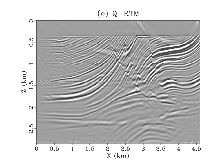
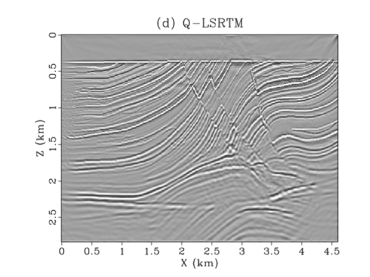
Figure 2: Comparison between images from (a) acoustic RTM, (b) acoustic LSRTM, (c) RTM using the visco-acoustic wave-equation, and (d) LSRTM using the visco-acoustic wave equation. The LSRTM images are after 20 iterations.
|
Required Software:
- Compilers: ifort/11.1.075, intel/15, mpi-openmpi/1.8.3-intel-15.
- Visualization: Madagascar-1.6.5.
Procedure:
- Load q_lsrtm.zip,
from which extract all the files to your working directory. (use "tar -xvf
q_lsrtm.tar.gz" to extract all the files). It includes following directories: source for the source codes, geom for the acquisition coordinates, model for the velocity models, modeling for the observed data and rtm for the rtm results.
- cd to the source directory and type "make" in the command terminal. This should compile all the codes. The executable is saved in the bin directory in the same folder.
- Description of some of the important codes in this directory:
- Makefile: Makefile for compiling all the codes.
- Makefile.config : Compiler flags to be used during the compilation.
- mmi.f90 : The main subroutine which decides the type of application to be executed.
- parser.f90,io.f90 : Subroutines for I/O and fetching parameters from the parameter files.
- mmi_mpi.f90 : MPI subroutines for the applications.
- datatype.f90 : Definition of the datatypes used.
- a2d_atten.f90.f90,a2d_staggered.f90 : Kernels for finite-difference simulation of the first-order visco-acoustic and acoustic wave equations.
- lsm_utilities.f90,lsm_utilities_staggered.f90 : Subroutines for computing the gradient, the step-length, updating the search direction using conjugate gradient, and preconditioning.
- apps2d_atten.f90,apps2d_lsm_staggered.f90 : Applications for doing Q-LSRTM and acoustic LSRTM.
- cd to the ../modeling directory and type "sbatch job_script_modeling.sh". This should generate the observed data (stored in the directory CSG) that will be used during the inversion. You have to configure this job script based on your cluster/workstation requirements.
- cd to the ../rtm directory and type "sbatch job_script_lsrtm.sh". This should generate the acoustic LSRTM images. The images are saved in the folder acoustic_lsrtm in the same directory. You have to configure this job script based on your cluster/workstation requirements.
- To view the acoustic RTM image, type "sfgrey < acoustic_lsrtm/mig_final_iter1.H title='(a) Acoustic RTM' pclip=95 label1=Z label2=X unit1=km unit2=km wheretitle=top wherexlabel=bottom labelsz=10 titlesz=12 titlefat=4 labelfat=4 | sfpen &". You should be able to see the image shown in Figure 2(a) above.
- To view the acoustic LSRTM image, type "sfgrey < acoustic_lsrtm/mig_final_iter20.H title='(b) Acoustic LSRTM' pclip=95 label1=Z label2=X unit1=km unit2=km wheretitle=top wherexlabel=bottom labelsz=10 titlesz=12 titlefat=4 labelfat=4 | sfpen &". You should be able to see the image shown in Figure 2(b) above.
- Type "sbatch job_script_qlsrtm.sh" in the command terminal. This should generate the Q-LSRTM images. The images are saved in the folder q_lsrtm in the same directory. You have to configure this job script based on your cluster/workstation requirements.
- To view the Q-RTM image, type "sfgrey < q_lsrtm/mig_final_iter1.H title='(c) Q-RTM' pclip=95 label1=Z label2=X unit1=km unit2=km wheretitle=top wherexlabel=bottom labelsz=10 titlesz=12 titlefat=4 labelfat=4 | sfpen &". You should be able to see the image shown in Figure 2(c) above.
- To view the Q-LSRTM image, type "sfgrey < q_lsrtm/mig_final_iter20.H title='(d) Q-LSRTM' pclip=95 label1=Z label2=X unit1=km unit2=km wheretitle=top wherexlabel=bottom labelsz=10 titlesz=12 titlefat=4 labelfat=4 | sfpen &". You should be able to see the image shown in Figure 2(d) above.
| |