|
Objective:
Learn how to do wave-equation Q tomography using the visco-acoustic wave-equation.
|
Required Software:
- Compilers: ifort/11.1.075, intel/15, mpi-openmpi/1.8.3-intel-15.
- Visualization: Madagascar-1.6.5.
Procedure:
- Load wq.tar.gz,
from which extract all the files to your working directory. (use "tar -xvf
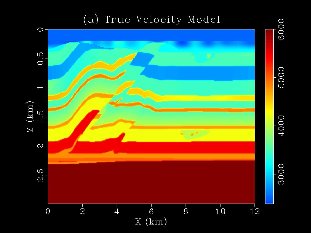
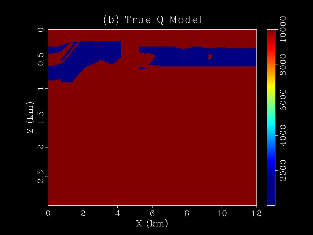
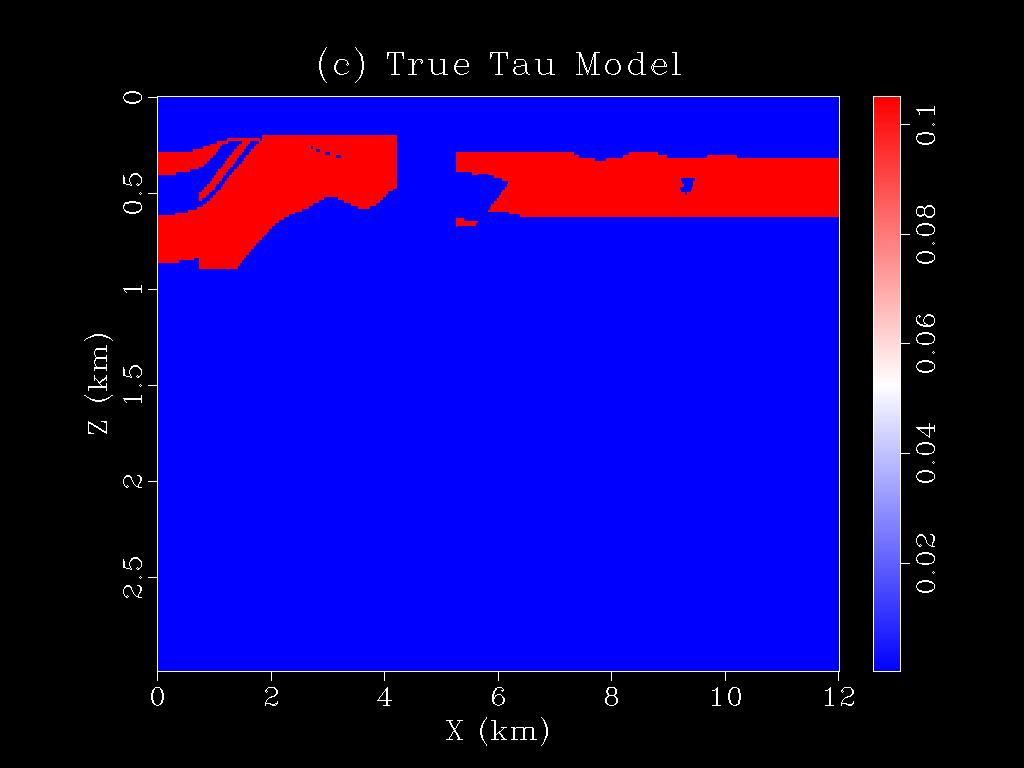
wq.tar.gz" to extract all the files). It includes following directories: src for the source codes, geom for the acquisition coordinates, model for the velocity models and wq for the WQ results.
- cd to the src directory and type "make" in the command terminal. This should compile all the codes. The executable is saved in the bin directory in the same folder.
- Description of some of the important codes in this directory:
- Makefile: Makefile for compiling all the codes.
- Makefile.config : Compiler flags to be used during the compilation.
- mmi.f90 : The main subroutine which decides the type of application to be executed.
- parser.f90,io.f90 : Subroutines for I/O and fetching parameters from the parameter files.
- mmi_mpi.f90 : MPI subroutines for the applications.
- datatype.f90 : Definition of the datatypes used.
- a2d_atten_wq.f90.f90 : Kernels for finite-difference simulation of the first-order visco-acoustic and acoustic wave equations.
- wq_utilities_atten_ssp.f90 : Subroutines for computing the gradient and the step-length.
- apps2d_wq_ssp.f90 : Application for doing WQ.
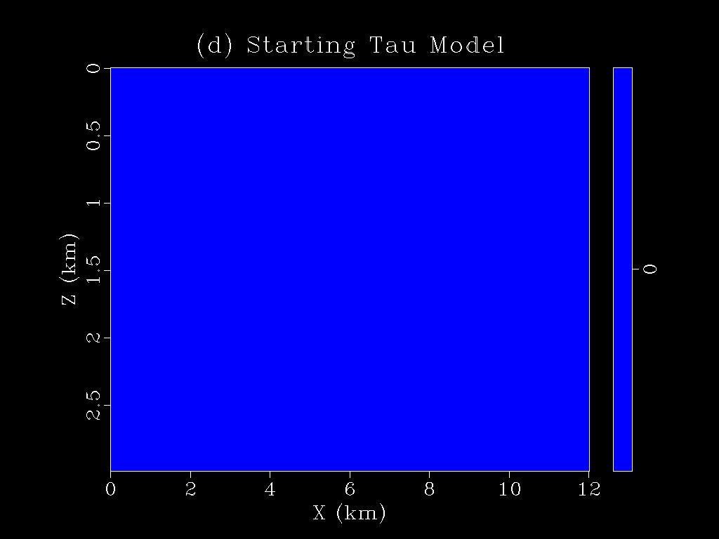
- cd to the ../wq directory and type "sbatch job_script_modeling.sh". This should generate the observed data (stored in the directory CSG) that will be used during the inversion. You have to configure this job script based on your cluster/workstation requirements.
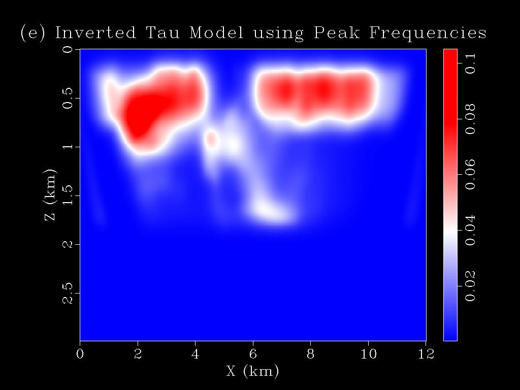
- Type "sbatch job_script_wq.sh". This should generate the WQ tomograms using the difference between the peak-frequency shifts between the observed and the predicted traces. You have to configure the job script based on your cluster/workstation requirements.
- The tomograms are saved in the folder tomograms in the same directory. To view them, type "sfgrey < tomograms/tau50.H bias=0.0002 color=E allpos=y label1='Z (km)' label2='X (km)' wherexlabel='bottom' title='(e) Inverted Tau Model using Peak Frequencies' wheretitle=top wantscalebar=y | sfpen" in the command terminal. This will generate Figure 1(e) shown above.
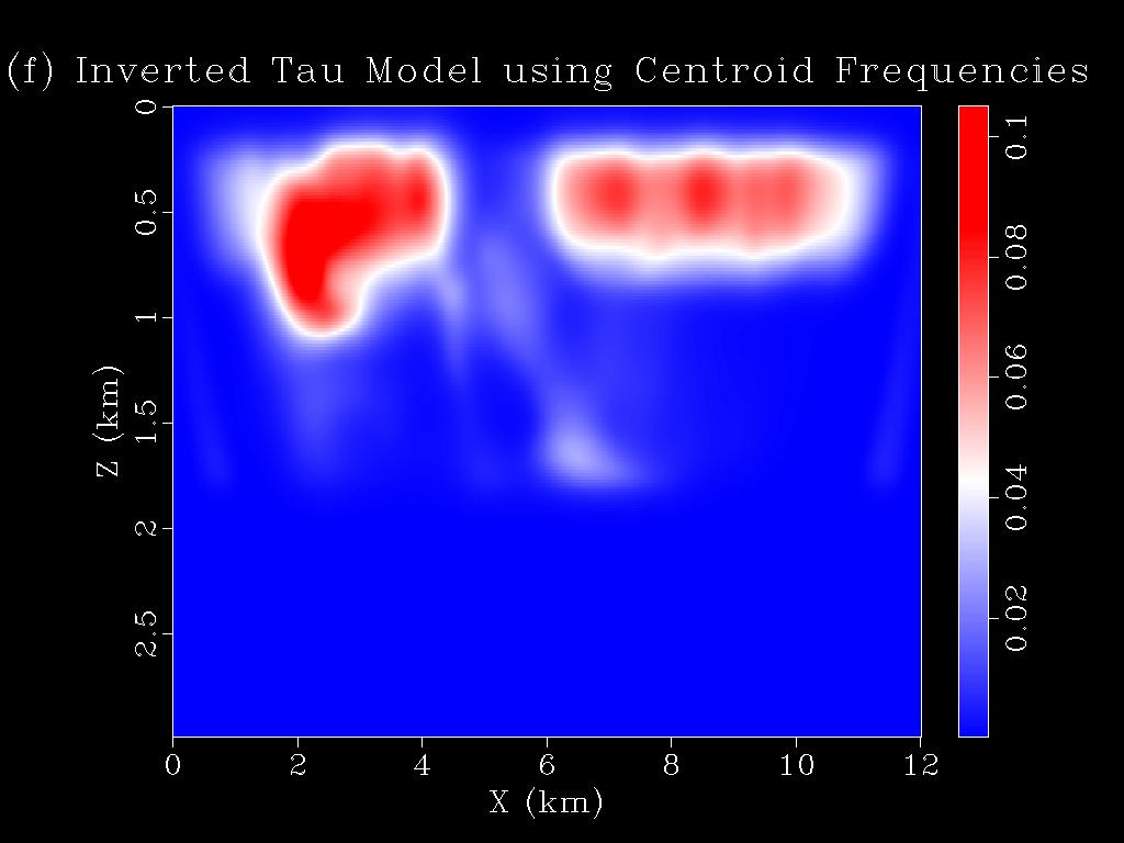
- Change the parameter "METHOD" in the parameter file "parfile_wq_ssp" from 1 to 2. Then type "sbatch job_script_wq.sh". This should generate the WQ tomograms using the difference between the centroid frequency shifts between the observed and the predicted traces. You have to configure the job script based on your cluster/workstation requirements.
- The tomograms are saved in the folder tomograms in the same directory. To view them type "sfgrey < tomograms/tau50.H bias=0.0002 color=E allpos=y label1='Z (km)' label2='X (km)' wherexlabel='bottom' title='(f) Inverted Tau Model using Centroid Frequencies' wheretitle=top wantscalebar=y | sfpen" in the command terminal. This will generate Figure 1(f) shown above.
- Copy the tomograms directory to your local workstation. If you can use Matlab in your cluster, you can skip this step.
- In Matlab command window, type "plot_wq.m". This will generate the Q models from the inverted Tau tomograms.
| |