CSIM Wave equation Series Lab
Part 1: TDFD solver to acoustic wave equation lab
PART 2: Reverse time migration lab
PART 3: Born modeling and adjoint test lab
PART 4: Wavepath lab
Objective:
Learn the adjoint operation of RTM, adjoint test and migration green's function.
Procedure:
- Define a 3 layer velocity model, and the model parameters;
vel=[repmat(1000,[1,30]), repmat(1200,[1,30]), repmat(1500,[1,21])];
vel=repmat(vel',[1 201]); [nz,nx]=size(vel); dx=5; x = (0:nx-1)*dx; z = (0:nz-1)*dx;
- Define the source and receiver geometry;
sx = (nx-1)/2*dx; sz = 0; gx=(0:2:(nx-1))*dx; gz=zeros(size(gx));
- Setup FD parameters and source wavelet;
nbc=40; nt=2001; dt=0.0005; t=(0:nt-1)*dt;isFS=false;freq=25; s=ricker(freq,dt);
- Smooth the true veolicyt to get the migration velocity model;
[vel_ss,refl_ss]=vel_smooth(vel,3,3,1);
- Plot the background velocity, reflectivity model and wavelet;
figure(2);set(gcf,'position',[0 0 1000 500]);colormap(gray);
subplot(231);imagesc(x,z,vel_ss);colorbar;
xlabel('X (m)'); ylabel('Z (m)'); title('smooth velocity');
figure(2);subplot(232);imagesc(x,z,refl_ss);colorbar;
xlabel('X (m)'); ylabel('Z (m)'); title('reflectivity');
figure(2);subplot(233);plot((0:numel(s)-1)*dt,s);
xlabel('Time (s)'); ylabel('Amplitude');title('wavelet');
- Run the modeling code, watch the movie of wave propagation including both background wave field and pertubation wave field, then plot the seismic data;
tic;seis=a2d_bmod_abc28_snapshot(vel_ss,refl_ss,nbc,dx,nt,dt,s,sx,sz,gx,gz,isFS);toc;
- Do the RTM with the generated born data;
% Forward Modeling to save BC
tic; [~,bc_top,bc_bottom,bc_left,bc_right,bc_p_nt,bc_p_nt_1]=...
a2d_mod_abc28(vel_ss,nbc,dx,nt,dt,s,sx,sz,gx,gz,isFS);toc;
% RTM
img=a2d_rtm_abc28(seis,vel_ss,nbc,dx,nt,dt,s,sx,sz,gx,gz,...
bc_top,bc_bottom,bc_left,bc_right,bc_p_nt,bc_p_nt_1);
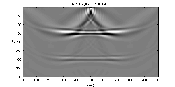
figure(3);set(gcf,'position',[0 0 600 300]);colormap(gray);
imagesc(x,z,img);caxis([-100 100]);
xlabel('X (m)'); ylabel('Z (m)'); title('RTM Image with Born Data');
- Adjoint test, since we have m, Lm and LTLm now, we will calculate LLTLm to examine our operator to see if they can pass the adjoint test.
tic;seis_new=a2d_bmod_abc28(vel_ss,img,nbc,dx,nt,dt,s,sx,sz,gx,gz,isFS);toc;
a=sum(refl_ss(:).*img(:));
b=sum(seis(:).^2);
c=sum(img(:).^2);
d=sum(seis(:).*seis_new(:));
display(['<Lm,Lm> = ',num2str(b)]);
display(['<m,LTLm> = ',num2str(a)]);
display(['<LTLm,LTLm> = ',num2str(c)]);
display(['<Lm,LLTLm> = ',num2str(d)]);
- Finally, calculate the migration greens function for a point scatterrer reflectivity model.
vel(:)=min(vel(:)); refl=zeros(size(vel)); refl((nz+1)/2,(nx+1)/2)=1;
[seis,bc_top,bc_bottom,bc_left,bc_right,bc_p_nt,bc_p_nt_1]...
=a2d_bmod_abc28(vel,refl,nbc,dx,nt,dt,s,sx,sz,gx,gz,isFS);
img=a2d_rtm_abc28(seis,vel,nbc,dx,nt,dt,s,sx,sz,gx,gz,...
bc_top,bc_bottom,bc_left,bc_right,bc_p_nt,bc_p_nt_1);
figure(4);set(gcf,'position',[0 0 600 800]);colormap(gray);
subplot(311);imagesc(x,z,vel);colorbar;
xlabel('X (m)'); ylabel('Z (m)'); title('Velocity');
figure(4);subplot(312);imagesc(x,z,refl);colorbar;
xlabel('X (m)'); ylabel('Z (m)'); title('Reflectivity');
figure(4);subplot(313);imagesc(x,z,img);caxis([-10 10]);
xlabel('X (m)'); ylabel('Z (m)'); title('Migration Greens Function');
Reminder:
For all labs, you can copy the bold line command to a single script, and run the scripts to generate the same results.
References:
- Seismic Inversion, Gerard T. Schuster
|