CSIM Wave equation Series Lab
Part 1: TDFD solver to acoustic wave equation lab
PART 2: Reverse time migration lab
PART 3: Born modeling and adjoint test lab
PART 4: Wavepath lab;
Objective:
Learn and run the time domain finite difference (TDFD) solver to the 2D acoustic wave equation.
Procedure:
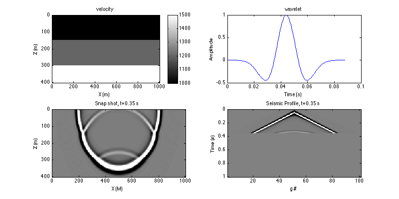
- Define a 3 layer velocity model, and the model parameters;
vel=[repmat(1000,[1,30]), repmat(1200,[1,30]), repmat(1500,[1,21])];
vel=repmat(vel',[1 201]);
[nz,nx]=size(vel); dx=5; x = (0:nx-1)*dx; z = (0:nz-1)*dx;
- Define the source and receiver geometry;
sx = (nx-1)/2*dx; sz = 0;
gx=(0:2:(nx-1))*dx; gz=zeros(size(gx));
- Setup FD parameters;
nbc=40; nt=2001; dt=0.0005;isFS=false;
- Setup the source wavelet;
freq=25; s=ricker(freq,dt);
- Plot the velocity and wavelet;
figure(1);set(gcf,'position',[0 0 800 400]);subplot(221);imagesc(x,z,vel);colorbar;
xlabel('X (m)'); ylabel('Z (m)'); title('velocity');
figure(1);subplot(222);plot((0:numel(s)-1)*dt,s);
xlabel('Time (s)'); ylabel('Amplitude');title('wavelet');
- Run the modeling code, watch the movie of wave propagation, and plot the seismic data;
tic;seis=a2d_mod_abc28_snapshot(vel,nbc,dx,nt,dt,s,sx,sz,gx,gz,isFS);toc;
Reminder:
For all labs, you can copy the bold line command to a single script, and run the scripts to generate the same results.
References:
- Seismic Inversion, Gerard T. Schuster
|