CSIM Wave equation Series Lab
Part 1: TDFD solver to acoustic wave equation lab
PART 2: Reverse time migration lab
PART 3: Born modeling and adjoint test lab
PART 4: Wavepath lab;
Objective:
Learn and run the reverse time migration code, see the difference of w/i and w/o direct wave, learn the impact of illumination compensation, and learn the basic of paralle matlab scripts.
Procedure:
- Single shot RTM;
- Define a 3 layer velocity model, and the model parameters;
vel=[repmat(1000,[1,30]), repmat(1200,[1,30]), repmat(1500,[1,21])];
vel=repmat(vel',[1 201]);[nz,nx]=size(vel); dx=5; x = (0:nx-1)*dx; z = (0:nz-1)*dx;
- Define the source and receiver geometry;
sx = (nx-1)/2*dx; sz = 0;
gx=(0:2:(nx-1))*dx; gz=zeros(size(gx)); ng=numel(gx); g=1:ng;
- Setup FD parameters and source wavelet;
nbc=40; nt=2001; dt=0.0005; t=(0:nt-1)*dt;isFS=false;freq=25; s=ricker(freq,dt);
- Calculate the seismic data by running the modeling code of part 1, use the true velocity model;
tic;seis=a2d_mod_abc28(vel,nbc,dx,nt,dt,s,sx,sz,gx,gz,isFS);toc;
- Smooth the true veolicyt to get the migration velocity model;
[vel_ss,refl_ss]=vel_smooth(vel,3,3,1);
- Plot the velocity and seismic data;
figure(3);set(gcf,'position',[0 0 1000 400]);subplot(231);imagesc(x,z,vel);colorbar;
xlabel('X (m)'); ylabel('Z (m)'); title('velocity');
figure(3); subplot(232);imagesc(g,t,seis);colormap(gray);
title('Seismic Profile');ylabel('Time (s)');xlabel('g #');caxis([-0.25 0.25]);
- Run the rtm code, watch the movie of forward propagation field, reconstruction forward field, backward propagation field and accumulated rtm image;
tic;[img,illum]=a2d_rtm_abc28_snapshot(seis,vel_ss,nbc,dx,nt,dt,s,sx,sz,gx,gz);toc;
- Plot the illumination compensation, and see the impact.
figure(4); set(gcf,'position',[0 0 400 600]);colormap(gray);
subplot(311);imagesc(x,z,img);caxis([-10 10]);
xlabel('X (m)'); ylabel('Z (m)'); title('rtm image');
figure(4);subplot(312);imagesc(x,z,illum);caxis([-100 100]);
xlabel('X (m)'); ylabel('Z (m)'); title('illumination compensation');
figure(4);subplot(313);imagesc(x,z,img./illum);caxis([-1 1]);
xlabel('X (m)'); ylabel('Z (m)'); title('rtm image after compensation');
- Mute the direct wave, and rerun the migration.
vel_homo=zeros(size(vel))+min(vel(:));
tic;seis_homo=a2d_mod_abc28(vel_homo,nbc,dx,nt,dt,s,sx,sz,gx,gz,isFS);toc;
figure(3);set(gcf,'position',[0 0 1000 400]);subplot(231);imagesc(x,z,vel);colorbar;
xlabel('X (m)'); ylabel('Z (m)'); title('velocity');
seis=seis-seis_homo;
figure(3); subplot(232);imagesc(g,t,seis);figure_title='Seismic Profile';
title(figure_title);ylabel('Time (s)');xlabel('g #');caxis([-0.25 0.25]);
[img,illum]=a2d_rtm_abc28_snapshot(seis,vel_ss,nbc,dx,nt,dt,s,sx,sz,gx,gz);
figure(5); set(gcf,'position',[0 0 400 600]);colormap(gray);
subplot(311);imagesc(x,z,img);caxis([-10 10]);xlabel('X (m)'); ylabel('Z (m)'); title('rtm image');
figure(5);subplot(312);imagesc(x,z,illum);caxis([-100 100]);xlabel('X (m)'); ylabel('Z (m)'); title('illumination compensation');
figure(5);subplot(313);imagesc(x,z,img./illum);caxis([-1 1]);xlabel('X (m)'); ylabel('Z (m)'); title('rtm image after compensation');
- All shots reverse time migration by parallel MATLAB;
- Initial the parallel mode;
parallel_init;
- Define the source and receiver geometry;
gx=(0:2:(nx-1))*dx; ng=numel(gx);
sx=(0:4:(nx-1))*dx; ns=numel(sx); sz=zeros(ns);
- Generate the syhthetic seismic data and mute the direct wave;
tic;seis=zeros(nt,ng,ns);display('Modeling to generate data');
parfor is=1:ns
display(['Modeling, is=',num2str(is),', ns=',num2str(ns)]);
seis(:,:,is)=a2d_mod_abc28(vel,nbc,dx,nt,dt,s,sx(is),sz(is),gx,gz,isFS);
seis_homo=a2d_mod_abc28(vel_homo,nbc,dx,nt,dt,s,sx(is),sz(is),gx,gz,isFS);
seis(:,:,is)=seis(:,:,is)-seis_homo;
end
- Forward propagate to save boundaries;
bc_top=zeros(5,nx,nt,ns); bc_bottom=zeros(5,nx,nt,ns);
bc_left=zeros(nz,5,nt,ns);bc_right=zeros(nz,5,nt,ns);
bc_p_nt=zeros(nz+2*nbc,nx+2*nbc,ns);bc_p_nt_1=zeros(nz+2*nbc,nx+2*nbc,ns);
display('Modeling to save BC');
parfor is=1:ns
display(['Modeling, is=',num2str(is),', ns=',num2str(ns)]);
[~,bc_top(:,:,:,is),bc_bottom(:,:,:,is),bc_left(:,:,:,is),...
bc_right(:,:,:,is),bc_p_nt(:,:,is),bc_p_nt_1(:,:,is)]...
=a2d_mod_abc28(vel_ss,nbc,dx,nt,dt,s,sx(is),sz(is),gx,gz,isFS);
end
- RTM
img=zeros(nz,nx,ns);illum=zeros(nz,nx,ns);
parfor is=1:ns
display(['RTM, is=',num2str(is),' ns=',num2str(ns)]);
[img(:,:,is),illum(:,:,is)]=a2d_rtm_abc28(seis(:,:,is),vel_ss,nbc,dx,nt,dt,s,sx(is),sz(is),gx,gz,...
bc_top(:,:,:,is),bc_bottom(:,:,:,is),bc_left(:,:,:,is),...
bc_right(:,:,:,is),bc_p_nt(:,:,is),bc_p_nt_1(:,:,is));
end
toc;
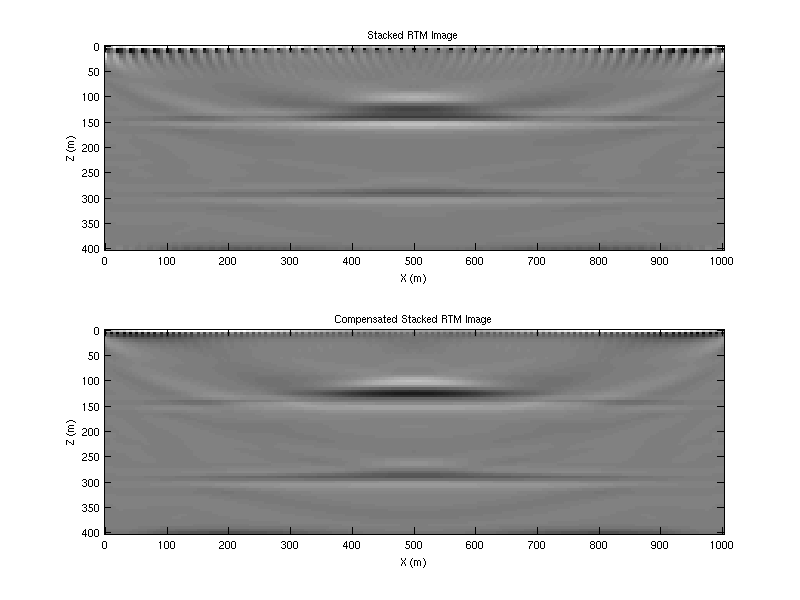
- Stack the prestack image, apply the highpass filter and plot the final results
image=sum(img,3);image_illum=sum(img./illum,3);
figure(6);set(gcf,'position',[0 0 800 600]);colormap(gray);
subplot(211);imagesc(x,z,highpass(image,10,2));caxis([-1000 1000]);
xlabel('X (m)'); ylabel('Z (m)'); title('Stacked RTM Image');
figure(6);subplot(212);imagesc(x,z,highpass(image_illum,10,2));caxis([-50 50]);
xlabel('X (m)'); ylabel('Z (m)'); title('Compensated Stacked RTM Image');
- Exit the parallel mode;
parallel_stop;
Reminder:
For all labs, you can copy the bold line command to a single script, and run the scripts to generate the same results.
References:
- Seismic Inversion, Gerard T. Schuster
|