Seismic Experiment at North Arizona

To Locate Washington Fault

1. 2D Field Text

· Data in MatLab format

· Data in dpik format

· Topography, Ascii format

· First arrival traveltime picks (Ascii)

· Final Tomogram (MatLab)

· Raypath density (MatLab)

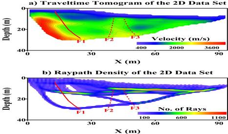
Figure (1): Upper is the traveltime tomogram and Lower is the raypath density

2. 3D Field Test

Data Acquisition

Short Video for data recording

Date: October 2008

Team: Sherif, Shendong, Xin Wang, Wei Dai, Joost, Bandar, Qiong, and Simmin

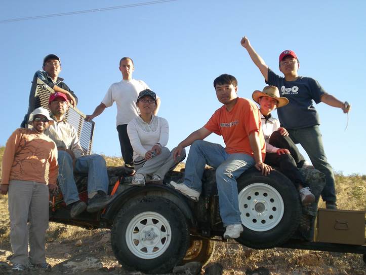
Figure (2): The team recorded the 3D seismic data at Washington Fault, Arizona

No. of receivers in the inline direction: 80

Number of lines: 6

Receiver Interval: 1 m near the fault, 2 m away from the fault (Receivers 1 to 12 at 2 m intervals, receivers 12 to 51 at 1 m intervals, and receivers 51 to 80 at 2 m intervals)

No. of shots in the inline direction: 40

Shot interval: 2 and 4 m (every other receiver location)

See Figure 3 and Shengdong master thesis for more details on the source/receiver locations

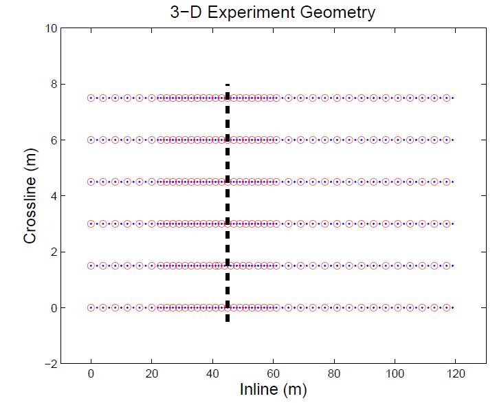
Figure (3): The 3D seismic experiment layout. The open circles are the source

locations and the blue dots are the receive locations

All details on this survey are in Shengdong thesis

The final tomogram is shown on Figure 4

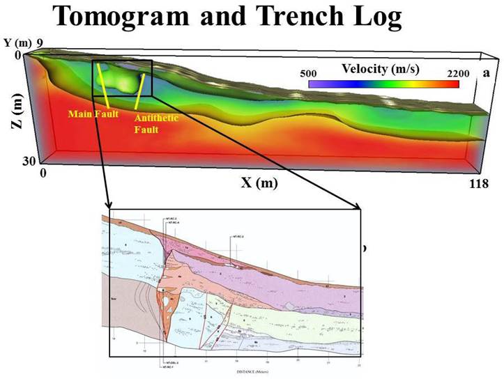
Figure (4): Upper is the 3D traveltime tomogram and the lower is the trench log

Data Recording

The data are recorded using two Bison equipment, each is 120 channels. We shot at all 240 shot locations and simultaneously recorded seismic traces at receivers 1 to 240 (using both Bisons), then we shot again at all 240 shot locations and we recorded at receivers 241 to 480.

The data is rearranged to match the receiver order shown in Figure 3 where receiver 1 is at left-lower corner, receivers increase to 80 at right lower corner, then receiver 81 is back to left side at Y = 1.5 m, etc.

Data is converted to matlab format and dpick format

1. Matlab format, sample interval is 0.25 ms, total number of samples/trace = 2000, total recording time = 0.5 s

2. DPick format (Part 1 CSG1-CSG60, Part 2 CSG61-CSG120, Part 3 CSG121-CSG180, and Part 4 CSG181-CSG240), resampled so that sample interval is 1 ms, total number of samples/trace = 500, and total recording time = 0.5 s

3. 3D Data Interpolation

The recorded data is interpolated using sinc technique to create the following two data sets

1. Data Set # 1: Here, we interpolated only in the receiver direction to regularize the receiver interval to 1 m, however, the source locations are the same as the original data (2 and 4 m source intervals). Now the data contains 6 lines, each line has 121 receivers and a total of 240 shot gathers. To download the data in MatLab format, please click here.

2. Data Set # 2: Here, we used the result from the previous step, and interpolated only in the shot direction to regularize the shot interval to 1 m. Now, both shot and receivers has 1 m interval. The data contains 6 lines, each line has 121 receivers and a total of 726 shot gathers. To download the data in MatLab format, please click here.