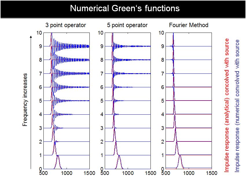
Figure 1. Comparison of 3-pt, 5-pt, and pseudospectral
solutions to the wave equation for different peak frequencies of the
source wavelet and a fixed dx interval. The horizontal axis is time
in units of time steps (adapted from Heiner Igel's PPT).
2D 2-8 FD Acoustic Modeling Lab (Xin Wang)
OBJECTIVE: Generate synthetic acoustic data with a MATLAB script
that solves the acoustic wave equation with a 2-8 FD method.
PROCEDURE:
- Load into your working directory
main.m,
a2d_mod_abc28.m,
ricker.m,
AbcCoef2D.m.
- Type the main code while in MATLAB. Snapshots will be playing for waves propagating in
a 2D layered medium. Finally a common shot gather will be displayed.
- Load the 2-4 accuracy code a2d_mod_abc24.m into your directory,
Similar to Figure 1, compare the 2-8 accuracy to the 2-4 accuracy after
propagating 40 wavelengths in a homogeneous medium (change velocity model to a homogeneous one in main.m).
- Change the boundary conditions grid number to a larger and smaller number, to see the absorbing effection.
- Change the boundary conditions to hybrid ABCs to absorb more effectively.
- Follow the example of 2-4 and 2-8 order FD code, write a 26 accuracy code.
The coefficients are c1 = -49.0/18.0, c2 = 3.0/2.0, c3 = -3.0/20.0 and c4 = 1.0/90.0.
Compare your results with the 2-4 and 2-8 in a homogeneous model.
- Change dx and dt, to see how to satisfy the stability condition.