CSIM Full Waveform Inversion Lab
By Xin Wang, Bldg 1, 3139-WS13, 808-0386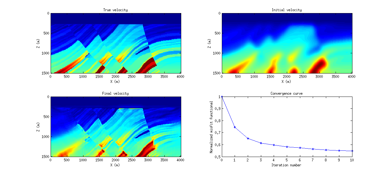
|
Objective:
Theory:
f = 0.5 * || A(s) - dobs || 2 The iterative procedures can be described as Procedure:
Questions:
|
CSIM Full Waveform Inversion Lab
By Xin Wang, Bldg 1, 3139-WS13, 808-0386
Objective:
Learn and explore the full waveform inversion.
Theory:
Assume the non-linear modeling operator is A(s), s is the slowness model, a initial slowness model is s0, and the observed data is dobs, the full waveform inversion algorithm is a iterative process to find a velocity model s to minimize the misfit functional:
f = 0.5 * || A(s) - dobs || 2
The iterative procedures can be described as
- Calculate the data misfit function with the initial slowness model
f = 0.5 * || A(s0) - dobs || 2;
- Apply the reverse time migration (RTM) operator LT to the data residual A(s) - dobs and get the gradient g1
- Find the conjugate direction for the current iteration:
c1 = g1 + <g1, g1>/<g, g> * c0,
where g0 is the gradient from last iteration, and c0 is the conjugate direction from last iteration;
- Give the trial step length alpha with, use the back tracking and hyperbolic interpolation to find the numerical step length gama * alpha
- Update the new slowness model:
s1 = s0 + alpha * gama * c1;
- Refresh the conjugate direction, gradient and the slowness model by:
c = c1;
g = g1;
s0 = s1;
- Repeat steps 1 to 6 until the procedures meets the designed iteration number or convergent criteria.
Procedure:
- Download FWI_LAB.tar.gz, and read and write MATLAB codes. extract the compressed package by tar -xvf FWI_LAB.tar.gz.
- Add the current directory to your MATLAB working path by addpath((genpath(pwd))) ;
- Go to the working directory by cd FWI_LAB;
- Comment lines 14 and 15 in fwi_modeling.m, and also change the command "n2s(is)" into "num2str(is)" in lines 39 and 40. Then o then run fwi_modeling to generate the synthetic data with the true cutted marmousi2 model;
- Comment lines 16 and 140 in fwi_debug.m. Read fwi.m or fwi_debug.m first and see how the FWI theory is implemented in the scripts;
- Comment lines 16 and 140 in fwi_debug.m. Run fwi_debug.m to apply FWI to the modeled data;
- Run fwi_plot to plot the results.
Questions:
- In this FWI approach, we mute the direct wave, what is the advantage and disadvantage if we include the direct wave?
- We limit the maximum and minimum velocity by v1(v1<vmin)=vmin;v1(v1>vmax)=vmax, why?
- If the starting velocity is far from the true, which results in a slow convergence, how can we speed it up?
- Choose another velocity model, design the acquisition geometry and the initial velocity model, run the FWI code and compare the results to see it works, if doesn't, why?
References:
- Seismic Inversion, Gerard T. Schuster