Prestack Least Squares Migration Lab (Fortran 90)
By Xin Wang (xin.wang@kaust.edu.sa), Bldg 1, 3139-WS13, 808-0386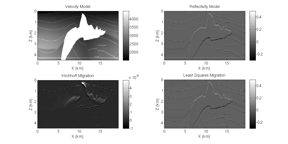
figure 1, Least squares migration of 2D SEG/EAGE salt model.
|
Objective:
Procedure:
References:
|
Prestack Least Squares Migration Lab (Fortran 90)
By Xin Wang (xin.wang@kaust.edu.sa), Bldg 1, 3139-WS13, 808-0386
figure 1, Least squares migration of 2D SEG/EAGE salt model.
Objective:
Build the least squares migration code with FORTRAN 90 from the given subroutines, use booth steepest descent (SD) and conjugate gradient (CG) methods, and practice with FORTRAN.
Procedure:
- Load lsm2d.tar, from which extract all files to your working directory. (use "tar -xvf lsm2d.tar" to extract file).
- Modify the main code "lsm2d.f90" to build your own LSM code. The procedure will be
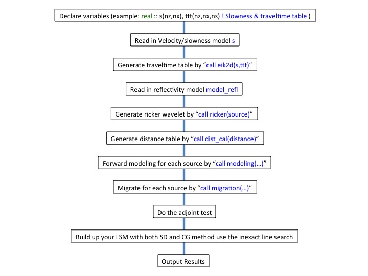
You will find in the "lsm2d.f90": most of the procedures have been written, the main work will be last three steps.
- Once you finished codeing, type "make" to compile your code, and type "make run" to execute your program. (Notice: you have to compile and run your code on the Linux workstation in RM 2220, Bldg 9, or any KAUST Linux workstation.)
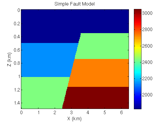
- Show your work with the "Simple Fault" Model, as shown in Figure 2.
figure 2. "Simple Fault" velocity model.
Show the migration image and LSM image for both SD and CG method, show your normalized convergence curve. Does your code pass the adjoint test? how much difference between those two terms?
- Change your background velocity to another one different from the true velocity, show your chosen background velocity model, migration image and LSM image, as well as the convergence curve, analysize your result (Tips:generate your data with the true velocity model, but do the migration and LSM with your chosen velocity model.)
- Show your work with the 2D SEG/EAGE salt model, as shown in Figure 1. (replace the lsm2d_parameters.par with lsm2d_parameters.par_seg, and change the input file name for both velocity model and reflectivity model). Show your migration image and LSM image with both CG and SD method. Compare with the LSM image, what is the main problem of the migration image? Show your normalized convergence curve.
- In CG method, reset the conjugate direction to the gradient for every 5 iterations, compare the result to CG without resetting, show the convergence curve and analysize your result.
References:
- Fortran 90 Handbook: Complete Ansi/Iso Reference (Computing That Works)
Jeanne C. Adams (Author), Walter S. Brainerd (Author), Jeanne T. Martin (Contributor)