Reverse Time Migration Lab
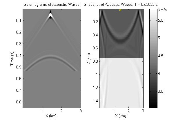
Figure 1.Seismograms and snapshot associated with a point source at the center of the surface in the 2-layer medium.
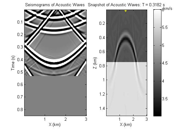
Figure 2. Back propagating wave field calculated by reversely inputting the calculated seismograms.
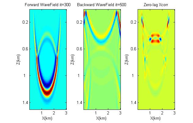
Figure 3. Zero-lag cross correlation (nt =800, for forward wave field it = 300, for backward wave field it = 500).
Objective: Calculate synthetic seismograms, forward wave field and back propagating wave field by a 2-4 FD solution to the wave equation for a point source at the surface. Adjust code so the data recorded at the surface is migrated by reverse time migration over all the shots.
Skill Learned: The idea of RTM; the implementation of RTM on very simple model and the parallelization of RTM.
Model used: A two-layered medium with velocity 4 km/s for the upper layer and velocity 5.6 km/s for the lower layer.
Procedure:
- Download the supporting codes plt.m, Laplacian.m and save_survey.m and create two new directories fd_data and bk_data under the current directory ./.
- Download the major codes fd.m, bkwd.m and rtm.m and type "fd". This will generate the synthetic seismograms and snapshots for a 2-layer medium.
- Type "bkwd" to generate back propagating wave field.
- Type "rtm" to sum up zero-lag xcorr over every time iteration for one shot.
Exercises:
- Run fd.m to generate the forward seismogram and wave field Why do we save the forward wave field for each iteration?
- Run bkwd.m to generate the backward wave field? What is the physical meaning of the backward wave field (i.e. Figure 2)?
- Do rtm.m for one shot. What is the meaning of the dot product (i.e. Figure 3)?
- Parallelizing the fd.m bk.m and rtm.m codes by uncommenting "matlabpool local", "parfor is = ... " and commenting "for is = ... ". This is doing RTM for all the shots. You can design your own shots, i.e. number of shots and their locations.