RTM: Fault Model (MATLAB and 2-2 FD)
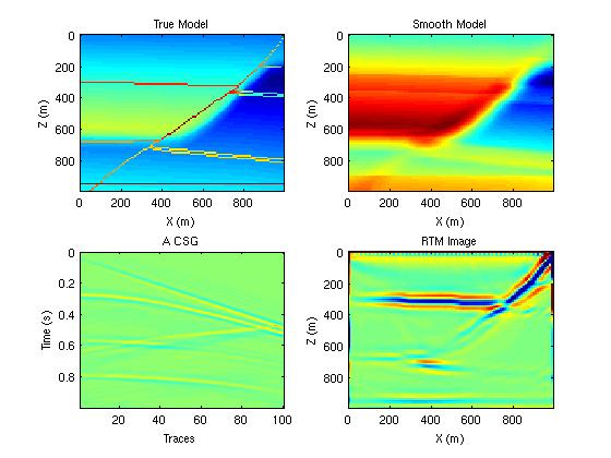
Figure 1. a) True model. b) The smooth background model. c) an example CSG. d) The RTM image.
Objective: Calculate synthetic seismograms by a 2-2 FD solution to the
wave equation for a point source, then migrate the recorded data with a smooth background velocity model and post-process the RTM image to remove the strong surface artifacts.
Skill Learned: Implementation, design and construction of simple RTM code.
Introduction:
The perfectly matching layers are placed at all four boundaried of the model to absorb outgoing waves, so there is no free surface reflection. Each migration contains 3 FD simulations: forward propagating of forward field, backward propagating of forward field and backward propagating of backward field. The dot production imaging condition is applied during the backward propagating at each time step.
A Laplacian filter is applied to the RTM image as a post-processing step to remove the low wavenumber artifacts.
Procedure:
- Download the codes fmod.m ,rtm.m , plt2.m and vel.dat and type "fmod". This will generate the synthetic seismograms and save them in a file csg.bin. Type "rtm". to migrate the recorded data.
Exercises:
- Run the code to generate synthetic data and migrate them. Examine the quality of the image. Run plt.m to filter the image with a Laplacian filter and compare the difference.
- The direct wave in the recorded data should be muted to remove part of the strong shallow artifacts. This can be done in two ways: 1. use a ray tracing program and predict the arrival time of the direct wave, then mute the direct wave. 2. do forward modeling with the smooth background velocity model to generate another dataset and subtract it from the recorded data. The 2nd method is used in rtm.m ( uncomment line 303 ).
- Comment out the part where the velocity is smoothed in rtm.m (line 38-57, and line 303), so that the true velocity model is used to migrate the recorded data. Filter the RTM image with the Laplacian filter and compare it with the image generated in step 1.
- Adjust the program to run the same simulations with the full model in velvector. Use the same tricks to mute the direct wave and post-process the images also.