CSIM Wave equation Series Lab
Part 1: TDFD solver to acoustic wave equation lab
PART 2: Reverse time migration lab
PART 3: Born modeling and adjoint test lab
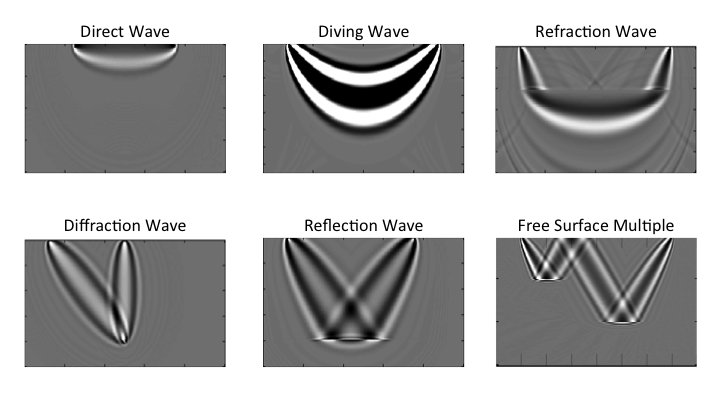
PART 4: Wavepath lab
Objective:
Learn and discuss the wave path of different type of waves.
Theory:
- For direct, diving and refraction wave, just use the conventional rtm code and mute other events but only themselves left:
WP = P • Q
P is the forward propagation field, and Q is the backward propagation field.
- For reflection and diffraction wave, a reflectivity model and an additional born modeling is needed:
WP = P • PP
+ Q • QQ
PP is the backward pertubation field, which is calculated by a born modeling of the pertubated reflectivity and the background wave field Q;
and QQ the forward pertubation field, which is calculated by a born modeling of the pertubated reflectivity and the background wave field P.
Procedure:
- Direct wave wavepath
- Define a homogenerous velocity model, and the model parameters;
nz=81;nx=201;vel=zeros(nz,nx)+1000; dx=5;
x = (0:nx-1)*dx; z = (0:nz-1)*dx;
- Define the source and receiver geometry;
sx = (nx-1)/4*dx; sz = 0; gx=(0:2:(nx-1))*dx; gz=zeros(size(gx)); g=1:numel(gx);
- Setup FD parameters and source wavelet;
nbc=40; nt=2001; dt=0.0005; t=(0:nt-1)*dt;isFS=false;freq=25; s=ricker(freq,dt);
- Generate the synthetic data;
tic; seis=a2d_mod_abc28(vel,nbc,dx,nt,dt,s,sx,sz,gx,gz,isFS);toc;
- Calculate and plot the wavepath for direct wave;
figure(1);set(gcf,'position',[0 0 1000 500]);
subplot(221);imagesc(x,z,vel);colorbar;xlabel('X (m)'); ylabel('Z (m)'); title('velocity');
figure(1);subplot(222);imagesc(g,t,seis);colormap(gray);
xlabel('Time (t)'); title('seismic gather');
figure(1);subplot(223);plot(t,seis(:,76));xlabel('Time (t)'); title('seismic trace');
tic; wp=a2d_wavepath_abc28(seis(:,76),vel,nbc,dx,nt,dt,s,sx,sz,gx(76),gz(76)); toc;
figure(1);subplot(224);imagesc(x,z,wp);colormap(gray);caxis([-10 10]);
xlabel('X (m)'); ylabel('Z (m)'); title('wave path for direct wave');
- Diving wave wavepath
- Define a gradient velocity model, and the model parameters;
vel=(1000:1000/150:2000);vel=repmat(vel',[1,401]);
[nz,nx]=size(vel);x = (0:nx-1)*dx; z = (0:nz-1)*dx;
- Define the source and receiver geometry;
sx = (nx-1)/8*dx; sz = 0; gx=(0:2:nx-1)*dx; gz=zeros(size(gx)); g=0:numel(gx);
- Setup FD parameters and source wavelet;
nbc=40; nt=4001; dt=0.0005; t=(0:nt-1)*dt;isFS=false;freq=25; s=ricker(freq,dt);
- Generate the synthetic data;
tic; seis=a2d_mod_abc28(vel,nbc,dx,nt,dt,s,sx,sz,gx,gz,isFS);toc;
- Calculate and plot the wavepath for diving wave;
figure(2);set(gcf,'position',[0 0 1000 500]);
subplot(221);imagesc(x,z,vel);colorbar;
xlabel('X (m)'); ylabel('Z (m)'); title('velocity');
figure(2);subplot(222);imagesc(g,t,seis);colormap(gray);caxis([-1 1]);
xlabel('Time (t)'); title('seismic gather');
gx=gx(176);gz=gz(176); trace=seis(:,176); trace(2901:end)=0;
figure(2);subplot(223);plot(t,trace);
xlabel('Time (t)'); title('seismic trace with direct wave muted');
tic; wp=a2d_wavepath_abc28(trace,vel,nbc,dx,nt,dt,s,sx,sz,gx,gz); toc;
figure(2);subplot(224);imagesc(x,z,wp);colormap(gray);caxis([-0.1 0.1]);
xlabel('X (m)'); ylabel('Z (m)'); title('wave path for diving wave');
- Refraction wave wavepath
- Define a two layer velocity model, and the model parameters;
vel=[repmat(1000,[1 41]),repmat(2000,[1,80])];vel=repmat(vel',[1,401]);
[nz,nx]=size(vel);x = (0:nx-1)*dx; z = (0:nz-1)*dx;
- Define the source and receiver geometry;
sx = (nx-1)/8*dx; sz = 0; gx=(0:2:nx-1)*dx; gz=zeros(size(gx)); g=0:numel(gx);
- Setup FD parameters and source wavelet;
nbc=80; nt=4001; dt=0.0005; t=(0:nt-1)*dt;isFS=false;freq=25; s=ricker(freq,dt);
- Generate the synthetic data, and mute events other than refraction.
tic; seis=a2d_mod_abc28(vel,nbc,dx,nt,dt,s,sx,sz,gx,gz,isFS);toc;
trace=seis(:,176); trace(2801:end)=0;
- Calculate and plot the wavepath for refraction wave;
figure(3);set(gcf,'position',[0 0 1000 500]);
subplot(221);imagesc(x,z,vel);colorbar;xlabel('X (m)'); ylabel('Z (m)'); title('velocity');
figure(3);subplot(222);imagesc(g,t,seis);colormap(gray);caxis([-0.025 0.025]);xlabel('Time (t)'); title('seismic data');
figure(3);subplot(223);plot(t,trace);xlabel('Time (t)'); title('refraction wave');
tic; wp=a2d_wavepath_abc28(trace,vel,nbc,dx,nt,dt,s,sx,sz,gx(176),gz(176)); toc;
figure(3);subplot(224);imagesc(x,z,wp);colormap(gray);caxis([-0.0002 0.0002]);
xlabel('X (m)'); ylabel('Z (m)'); title('wave path for refraction wave');
- Diffraction wave wavepath
- Define a point scatterrer model, and the model parameters;
vel=zeros(101,201)+1000; vel(81,101)=1200;[nz,nx]=size(vel);x = (0:nx-1)*dx; z = (0:nz-1)*dx;
- Define the source and receiver geometry;
sx = (nx-1)/8*dx; sz = 0; gx=(0:2:nx-1)*dx; gz=zeros(size(gx)); g=0:numel(gx);
- Setup FD parameters and source wavelet;
nbc=80; nt=2601; dt=0.0005; t=(0:nt-1)*dt;isFS=false;freq=20; s=ricker(freq,dt);
- Smooth the background velocity;
[vel_ss,refl_ss]=vel_smooth(vel,3,3,1);
- Generate the synthetic data, and mute events other than diffraction.
tic; seis=a2d_mod_abc28(vel,nbc,dx,nt,dt,s,sx,sz,gx,gz,isFS);toc;
trace=seis(:,51); trace(1:1800)=0;trace(2301:end)=0;
- Calculate and plot the wavepath for diffraction wave;
figure(4);set(gcf,'position',[0 0 1000 500]);
subplot(221);imagesc(x,z,vel);colorbar;xlabel('X (m)'); ylabel('Z (m)'); title('velocity');
figure(4);subplot(222);imagesc(g,t,seis(1:2601,:));colormap(gray);caxis([-0.025 0.025]);
xlabel('Time (t)'); title('seismic data for one trace');
figure(4);subplot(223);plot(t,trace);xlabel('Time (t)'); title('diffraction wave');
tic; wp=a2d_wavepath_abc28_refl(trace,vel_ss,refl_ss,nbc,dx,nt,dt,s,sx,sz,gx(51),gz(51)); toc;
figure(4);subplot(224);imagesc(x,z,wp);colormap(gray);caxis([-0.002 0.002]);
xlabel('X (m)'); ylabel('Z (m)'); title('wave path for diffraction wave');
- Reflection wave wavepath
- Define a two layer model, and the model parameters;
vel=zeros(101,201)+1000; vel(81:end,:)=1500;[nz,nx]=size(vel);x = (0:nx-1)*dx; z = (0:nz-1)*dx;
- Define the source and receiver geometry;
sx = (nx-1)/8*dx; sz = 0; gx=(0:2:nx-1)*dx; gz=zeros(size(gx)); g=0:numel(gx);
- Setup FD parameters and source wavelet;
nbc=80; nt=2601; dt=0.0005; t=(0:nt-1)*dt;isFS=false;freq=20; s=ricker(freq,dt);
- Smooth the background velocity;
[vel_ss,refl_ss]=vel_smooth(vel,3,3,1);
- Generate the synthetic data, and mute events other than diffraction.
tic; seis=a2d_mod_abc28(vel,nbc,dx,nt,dt,s,sx,sz,gx,gz,isFS);toc;
trace=seis(:,76); trace(1:1800)=0;trace(2301:end)=0;
- Calculate and plot the wavepath for reflection wave;
figure(5);set(gcf,'position',[0 0 1000 500]);
subplot(221);imagesc(x,z,vel);colorbar;
xlabel('X (m)'); ylabel('Z (m)'); title('velocity');
figure(5);subplot(222);imagesc(g,t,seis(1:2601,:));colormap(gray);caxis([-0.1 0.1]);
xlabel('Time (t)'); title('seismic data for one trace');
figure(5);subplot(223);plot(t,trace);xlabel('Time (t)'); title('reflection wave');
tic; wp=a2d_wavepath_abc28_refl(trace,vel,refl_ss,nbc,dx,nt,dt,s,sx,sz,gx(76),gz(76)); toc;
figure(5);subplot(224);imagesc(x,z,wp);colormap(gray);caxis([-2 2]);
xlabel('X (m)'); ylabel('Z (m)'); title('wave path for reflection wave');
Reminder:
For all labs, you can copy the bold line command to a single script, and run the scripts to generate the same results.
References:
- Seismic Inversion, Gerard T. Schuster
|