Naoshi Aoki's Migration and Migration Velocity Lab

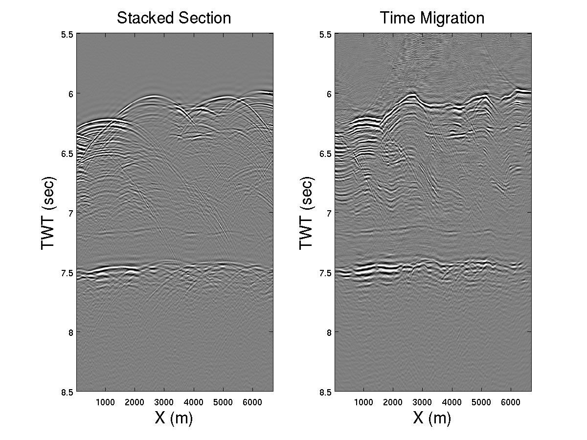
Figure 1: Stacked section (left) and migrated section (right) from the Nankai trough, offshore Japan.

We are going to process 2D seismic data* collected near the coast of Japan, over the Nankai trough, where the Philippines plate is subducting beneath Eurasia. The stacked section in Figure 1 shows many diffractions. Various migrations with different type of velocities will be applied to the data to acquire accurate structural image. The objectives of this lab are the followings:

l To be familiar with velocity terminology

l To learn what appropriate migration velocity is

*This data is obtained from the CDs with the book 'Seismic Data Processing with Seismic Un*x, SEG press'.

Procedure

1. Outlines, Codes, and Data

This lab consists of 4 parts: time migration with constant velocity, time migration with rms velocity, depth migration with straight ray assumption, and depth migration with eikonal traveltimes. Download MIGandMigVelLab.zip and uncompress it. You will find the following files:

The main code:

MigrationLabMain.m

You need the following codes to show stack section:

StraightRayDepthMigration.m

TimeMigrationLab.m

vintmod.m

The time migration with constant velocity lab:

TimeMigConst.m

timemigrate.m

The time migration with rms velocity lab requires:

TimeMigRms.m

timemigrate.m

vrmsmodel.m

The depth migration with straight ray assumption lab:

DepthMigStraightRay.m

vavemod.m

migrate_vave.m

The depth migration with eikonal traveltimes lab:

DepthMigEikonal.m

Slownessmod.m

Mray.m

In addition, traveltimes are already computed for your convenience.

TT.zip should be downloaded and uncompressed.

MandMVLab.zip is the entire lab and should be uncompressed.

2. Plot stack section

Execute code MigrationLabMain.m. The code shows stacked sections.

3. Time Migration with Constant Velocity

First we assume a homogeneous medium and will apply time migrations with constant velocities of 1500, 1550, 1600, 1650, and 1700 m/s. Comment out plotStack line on Line 40 in the main code, then uncomment TimeMigConst on Line 45. Execute MigrationLabMain again. Migration results will be shown. Compare migration images with different velocity and comment on that.

4. Time Migration with RMS Velocity

We will create time migration velocity (RMS velocity) from stacking velocity functions (also called NMO velocity functions). RMS velocity is defined by the following formula.

where Vint is interval velocity and is vertical traveltime within the interval. Stacking velocity functions can be obtained from velocity analysis. Stacking velocity is expected that it should be close to RMS velocity if the structure is not complicated.

Comment out TimeMigConst on Line 45 in the main code, then uncomment TimeMigRms on Line . Several functions picked by someone are available to use. Open vrmsmodel.m and you can see the velocity data. Since the data is sparse, we must gridding the data to use in migration. This code interpolates the velocity function and outputs 2 version of gridded velocity model, non-smoothed and smoothed. Execute MigrationLabMain again. Compare the time migration results with these velocities and comment on that.

5. Dix Inversion

Depth migration requires subsurface velocity model. Dix inversion is often used to estimate a velocity profile along seismic line. The following Dix equation inverts a vertical interval velocity between two picked seismic events:

where V_n is RMS velocity and t_n is the zero offset time. Then we obtain the thickness between the events:

where vertical traveltime. Note that the "interval" means not instantaneous velocity at some point but average velocity between adjacent picked points.

6. Depth migration with Straight Ray Assumption

We are going to apply depth migrations. Here we will take a straight ray assumption, where vertical ray does not bend and average velocity from any surface location to an image point is constant. This assumption is almost the same as time migration with RMS velocity case. The average velocity can be obtained from the following equation:

where Vint is gridded interval velocity model.

Now we comment out TimeMigrationLab in the main code, then uncomment DepthMigStraightRay. Open the sub code and the child code called vavemodel.m. The latter code shows a Dix interval velocity profile and outputs 2 versions of average velocity models, non-smoothed and smoothed, as same as the time migrations lab.

Execute the main code and acquire the results. Answer the following questions:

l Why depth migration result with non-smoothed velocity is so messy?

Hint: Over migration or migration smile will be observed when migration velocity is too fast.

l Do you believe this depth migration results? Why?

7. Depth Migration with Eikonal Traveltimes (Optional)

We are going to apply depth migration with traveltimes computed by eikonal solver Mray.m. Since the traveltime computation requires several hours to compute, the results are given in the directry called TT for your convenience. The file named TT_x.mat represents traveltime table at x location.

First comment out DepthMigStraightRay in the main code, then uncomment DepthMigEikonal. Open the code. Since the eikonal solver requires the same horizontal and vertical spacing, the vertical samples are decimated from nz to nzz. So we will interpolate traveltime in the depth migration code migrate_tt.m.

Note that Mray requires a gridded slowness model. Slowness is defined by:

where Vint represents a gridded interval velocity model. Slownessmod.m. creates a model from the smoothed interval velocity model.

Execute the main code. The code shows the slowness model and a movie of traveltimes. Then it migrates data with these traveltimes. Answer the the following:

l Is this better than the result from depth migration with straight ray assumption?
l Which is better, the time migration or the depth migration?
Why do the deeper horizontal layers appear thicker in the depth migration image compared to the shallower layers in the depth section? Why is this not true for the Time Migration Image?
If the velocity model is really complex e.g., a salt dome, which is the best migration method: time migration or depth migration? Why?
If the velocity model is mildly horizontal, which is the best migration method: time migration or depth migration? Why?
Which is faster, time migration or depth migration?
List the relative benefits and disadvantages of time vs depth migration.

Optional

1. Build a layered velocity model, which is your velocity structure interpretation, compute new traveltimes, and apply depth migration.

2. Create prestack depth migration code. Common shot gathers are available on the CDs with the book 'Seismic Data Processing with Seismic Un*x, SEG Press'.