Viscoacoustic Finite Difference Modeling using a SLS Model
Learn how to to do viscoacoustic forward modeling using staggered grids for a SLS model with a single relaxation mechanism, as shown here using Matlab®
Contents
Set up model parameters
clear all;
close all;
clc;

% Define model dimensions
nz=200; nx=200;
dx=10.0; dz=dx;

x=0:dx/1000:(nx-1)*dx/1000;
z=0:dz/1000:(nz-1)*dz/1000;

% Define the number of grid points used to pad the model boundaries
npml=40;

% Define size of the computational grid
nx_pml=nx+2*npml;
nz_pml=nz+2*npml;
Make background velocity, Q and density models
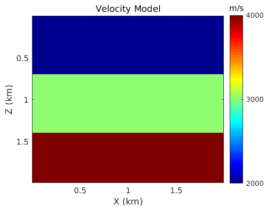
Make background velocity model.
c_tmp=3000*ones(nz,nx);
c_tmp(1:70,:)=2000;
c_tmp(71:140,:)=3000;
c_tmp(141:nz,:)=4000;

c=[repmat(c_tmp(:,1),1,npml), c_tmp, repmat(c_tmp(:,end),1,npml)];
c=[repmat(c(1,:),npml,1); c; repmat(c(end,:),npml,1)];

% Parameters used for plotting
title_fs=14; label_fs=12; axis_fs=12; cbar_fs=12; ifig=1; axis_fs=12;

% Plot the velocity model
figure; imagesc(x,z,c_tmp);
colormap('jet'); colorbar;
title('Velocity Model','FontWeight','Normal','FontSize',title_fs);
xlabel('X (km)','FontSize',12);
ylabel('Z (km)','FontSize',12);
sm_axis([0.5 1 1.5],[0.5 1 1.5],axis_fs);
h=colorbar; set(gca,'FontSize',cbar_fs);
set(h,'YTick',[2000 3000 4000])
text(2.05,-0.1,'m/s','FontSize',cbar_fs);

clear c_tmp;
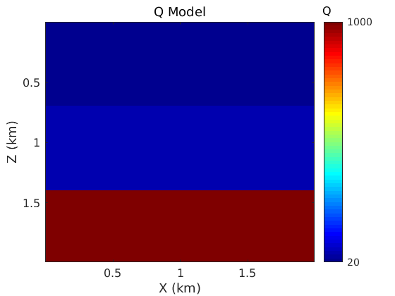
Make background Q model.
qf_tmp=20*ones(nz,nx);
qf_tmp(1:70,:)=20;
qf_tmp(71:140,:)=60;
qf_tmp(141:nz,:)=1000;

qf=[repmat(qf_tmp(:,1),1,npml),qf_tmp,repmat(qf_tmp(:,end),1,npml)];
qf=[repmat(qf(1,:),npml,1); qf; repmat(qf(end,:),npml,1)];

% Plot the Q model
figure; imagesc(x,z,qf_tmp); colormap('jet'); colorbar;
title('Q Model','FontWeight','Normal','FontSize',title_fs);
xlabel('X (km)','FontSize',12);
ylabel('Z (km)','FontSize',12);
sm_axis([0.5 1 1.5],[0.5 1 1.5],axis_fs);
h=colorbar; set(gca,'FontSize',cbar_fs);
set(h,'YTick',[20 1000])
text(2.05,-0.1,'Q','FontSize',cbar_fs);
clear qf_tmp;
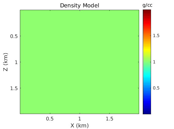
Make background density model. The density is taken to be constant in this lab.
den_tmp=ones(nz,nx);
den=[repmat(den_tmp(:,1),1,npml),den_tmp,repmat(den_tmp(:,end),1,npml)];
den=[repmat(den(1,:),npml,1); den; repmat(den(end,:),npml,1)];

% Plot the density model
figure; imagesc(x,z,den_tmp); colormap('jet'); colorbar;
title('Density Model','FontWeight','Normal','FontSize',title_fs);
xlabel('X (km)','FontSize',12);
ylabel('Z (km)','FontSize',12);
sm_axis([0.5 1 1.5],[0.5 1 1.5],axis_fs);
h=colorbar; set(gca,'FontSize',cbar_fs);
set(h,'YTick',[0.5 1 1.5])
text(2.05,-0.1,'g/cc','FontSize',cbar_fs);
clear den_tmp;
Define the number of time steps, the time sampling interval and the peak-frequency of the source wavelet used in the FD simulation.
nt=2000; dt=0.001; freq=20;
t=0:dt:(nt-1)*dt;
ns=50; ng=100;
Define the stress and strain relaxation parameters
The stress and strain relaxation parameters are given by
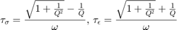
tausigma=(sqrt(1.0+1.0./qf.^2)-1.0./qf)./(2*pi*freq);
tauepsilon=(sqrt(1.0+1.0./qf.^2)+1.0./qf)./(2*pi*freq);
Damping coefficients at the model boundaries
Set up damping at the boundaries.
damp_global=zeros(nz_pml,nx_pml);
damp1=zeros(npml,1);

cmin=min(c(:));
a=(npml-1)*dx;
kappa = 3.0*cmin*log(10000000.0)/(2.0*a);
for ix=1:npml
  xa = real(ix-1)*dx/a;
  damp1(ix) = kappa*xa*xa;
end

for ix=1:npml
    for iz=1:nz_pml
        damp_global(iz,npml-ix+1)=damp1(ix);
        damp_global(iz,nx_pml+ix-npml)=damp1(ix);
    end
end

for iz=1:npml
    for ix=1+(npml-(iz-1)):nx_pml-(npml-(iz-1))
        damp_global(npml-iz+1,ix)=damp1(iz);
        damp_global(nz_pml+iz-npml,ix)=damp1(iz);
    end
end

clear damp1;
Generate Source Wavelet
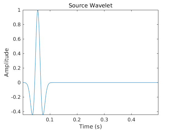
A Ricker wavelet with a peak frequency of 20 Hz is used as the source wavelet in the simulation.
s=ricker(freq,dt,nt);

figure; plot([0:499]*dt,s(1:500)); axis tight;
title('Source Wavelet','FontWeight','Normal','FontSize',14);
xlabel('Time (s)','FontSize',12);
ylabel('Amplitude','FontSize',12);
sm_axis([0.1 0.2 0.3 0.4 0.5],[-0.4 -0.2 0 0.2 0.4 0.6 0.8 1],axis_fs);
Set up acquisition geometry
% No of sources
ns=1;

% Source location in the model
isx=npml+1;
isz=npml+1;

% No of receivers
ng=nx;

% 8-th order staggered grid FD coefficients
c1_staggered_8th=1225.0/1024.0; c2_staggered_8th=-245.0/3072.0;
c3_staggered_8th=49.0/5120.0; c4_staggered_8th=-5.0/7168.0;

% Initialize the seismogram
seis=zeros(nt,ng);

% Memory allocations for the wavefields
u=zeros(nz_pml,nx_pml);
w=u; p=u; rl=u; rl1=u;
FD time marching loop
Time marching loop
for it=1:nt
Update the memory variable using the equation:
    rl1=rl;
    for ix=5:nx_pml-4
        for iz=5:nz_pml-4
            alpha=den(iz,ix)*c(iz,ix)*c(iz,ix)*dt*(tauepsilon(iz,ix)/tausigma(iz,ix)-1.0)/dx/tausigma(iz,ix);
            rl(iz,ix)=((1.0-dt/2.0/tausigma(iz,ix))*rl1(iz,ix)-alpha* ...
                       (c1_staggered_8th*(u(iz,ix)-u(iz,ix-1)+w(iz,ix)-w(iz-1,ix)) +   ...
                        c2_staggered_8th*(u(iz,ix+1)-u(iz,ix-2)+w(iz+1,ix)-w(iz-2,ix)) +   ...
                        c3_staggered_8th*(u(iz,ix+2)-u(iz,ix-3)+w(iz+2,ix)-w(iz-3,ix)) +   ...
                        c4_staggered_8th*(u(iz,ix+3)-u(iz,ix-4)+w(iz+3,ix)-w(iz-4,ix))))/(1.0+dt/2.0/tausigma(iz,ix));
        end
    end
Update the pressure wavefield using the equation:
    for ix=5:nx_pml-4
        for iz=5:nz_pml-4
            alpha=den(iz,ix)*c(iz,ix)*c(iz,ix)*dt*tauepsilon(iz,ix)/dx/tausigma(iz,ix);
            kappa=damp_global(iz,ix)*dt;
            p(iz,ix)=(1.0-kappa)*p(iz,ix)-0.5*(rl(iz,ix)+rl1(iz,ix))*dt-alpha* ...
                     (c1_staggered_8th*(u(iz,ix)-u(iz,ix-1)+w(iz,ix)-w(iz-1,ix))+ ...
                      c2_staggered_8th*(u(iz,ix+1)-u(iz,ix-2)+w(iz+1,ix)-w(iz-2,ix))+ ...
                      c3_staggered_8th*(u(iz,ix+2)-u(iz,ix-3)+w(iz+2,ix)-w(iz-3,ix))+ ...
                      c4_staggered_8th*(u(iz,ix+3)-u(iz,ix-4)+w(iz+3,ix)-w(iz-4,ix)));
        end
    end
Add source to the pressure variable
p(isz,isx)=p(isz,isx)+dt*s(it);
Update the X-component of the particle velocity v_x:
    for ix=5:nx_pml-4
        for iz=5:nz_pml-4
            alpha=dt/(den(iz,ix)*dx);
            kappa=0.5*(damp_global(iz,ix)+damp_global(iz,ix+1))*dt;
            u(iz,ix)=(1.0-kappa)*u(iz,ix)-alpha*(c1_staggered_8th*(p(iz,ix+1)-p(iz,ix))+...
                                                 c2_staggered_8th*(p(iz,ix+2)-p(iz,ix-1))+...
                                                 c3_staggered_8th*(p(iz,ix+3)-p(iz,ix-2))+...
                                                 c4_staggered_8th*(p(iz,ix+4)-p(iz,ix-3)));
        end
    end
Update the Z-component of the particle velocity v_z:
    for ix=5:nx_pml-4
        for iz=5:nz_pml-4
          alpha=dt/(den(iz,ix)*dx);
          kappa=0.5*(damp_global(iz+1,ix)+damp_global(iz,ix))*dt;
          w(iz,ix)=(1.0-kappa)*w(iz,ix)-alpha*(c1_staggered_8th*(p(iz+1,ix)-p(iz,ix))+ ...
                                               c2_staggered_8th*(p(iz+2,ix)-p(iz-1,ix))+ ...
                                               c3_staggered_8th*(p(iz+3,ix)-p(iz-2,ix))+ ...
                                               c4_staggered_8th*(p(iz+4,ix)-p(iz-3,ix)));
        end
    end
Output pressure seismogram
    for ig=1:ng
        igx=npml+ig;
        igz=npml+1;
        seis(it,ig)=p(igz,igx);
    end
end
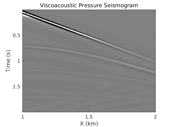
Plot the pressure seismogram
dg=dx/1000;
g=1:dg:nx*dg;

figure;
imagesc(g,t,seis./max(abs(seis(:))),[-0.01 0.01]); colormap('gray');
title('Viscoacoustic Pressure Seismogram','FontWeight','Normal','FontSize',title_fs);
xlabel('X (km)','FontSize',12);
ylabel('Time (s)','FontSize',12);
sm_axis([0.5 1 1.5 2],[0.5 1 1.5 2],axis_fs);
Homework Questions
1) Plot snapshots showing an expanding wavefront at different instances of time. Also, compare the snapshots with the snapshots in an acoustic medium. Comment on your observations.
2) Plot the depth/X-slices at different instances of time and comment on the amplitude and frequency loss of the propagating waves. Also, compare these slices with the slices in an acoustic medium.
3) Plot the amplitude spectra of a near-offset, a mid-offset and a far-offset trace and comment on what you infer from the spectra of these traces.
4) Derive the relaxation functions for a viscoelastic solid characterized by a single SLS mechanism.
5) Show a step-by-step derivation of the viscoelastic wave equation starting from the Hooke's law for an isotropic elastic solid.
6) Show that the viscoelastic wave equation reduces to the elastic wave equation when Qp and Qs becomes very large (the medium becomes lossless).
7) Modify the viscoacoustic wave equation code given in this lab for 3 SLS mechanisms. Compare the traces at the near-, mid- and far-offsets from the traces obtained using only 1 SLS. Comment on your observations.