Contents
Viscoelastic Finite Difference Modeling using a SLS Model
Learn how to to do viscoelastic forward modeling @version 1 2016-09-20 @author Bowen Guo & Zongcai Feng
% This is the main program to run viscoelastic modeling
% It involves function
%  staggerfd.m:   staggered grid finite difference
%  ricker.m:      generate ricker source wavelet
%  pad.m:         pad the model for absorbing boundary condition (ABC)
%  damp_circle.m  damp the padding zone of the model for ABC
%  calparam.m     calculate lambda and mu according to density, p/s velocity
Set up model parameters
clear all;
close all;
clc;

% Define model dimensions and source location
nx=302;dx=5.0;nz=302;dt=0.0003;dtx=dt/dx;
x=(0:nx-1)*dx/1000;
z=(0:nz-1)*dx/1000;
sx=nx/2;sz=nz/2;

% Make background P- and S-wave velocity, density models
vp=ones(nz,nx)*3000;
vs=vp/sqrt(3);
den=ones(nz,nx);

% Define the number of time steps, the time sampling interval and the peak-frequency of the source wavelet and absorb boudary paremeters
nt=round(min(nx,nz)/2*dx/(max(max(vp)))/dt);
fr=30;[source,nw]=ricker(fr,dt,nt);
nbc=max(max(vp))/fr/dx*2;
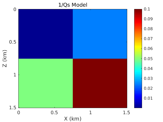
Make Qp and Qs models
%make Qp_rev=1/Qp
Qp_rev=ones(nz,nx);
Qp_rev(1:nz/2,1:nx/2)=Qp_rev(1:nz/2,1:nx/2)*0.00001;
Qp_rev(1:nz/2,nx/2+1:end)=Qp_rev(1:nz/2,nx/2+1:end)*0.025;
Qp_rev(nz/2+1:end,1:nx/2)=Qp_rev(nz/2+1:end,1:nx/2)*0.05;
Qp_rev(nz/2+1:end,nx/2+1:end)=Qp_rev(nz/2+1:end,nx/2+1:end)*0.1;
Qp=1./Qp_rev;

% Parameters used for plotting
title_fs=14; axis_fs=12; cbar_fs=12;

% Plot the Qp model
figure;
imagesc(x,z,Qp_rev); colormap('jet'); colorbar;
title('1/Qp Model','FontWeight','Normal','FontSize',title_fs);
xlabel('X (km)','FontSize',12);
ylabel('Z (km)','FontSize',12);
sm_axis([0 0.5 1 1.5],[0 0.5 1 1.5],axis_fs);
h=colorbar; set(gca,'FontSize',cbar_fs);
%set(h,'YTick',[0.0  0.1])
text(2.05,-0.1,'Q','FontSize',cbar_fs);

%make Qs_rev=1/Qs
Qs_rev=ones(nz,nx);
Qs_rev(1:nz/2,1:nx/2)=Qs_rev(1:nz/2,1:nx/2)*0.00001;
Qs_rev(1:nz/2,nx/2+1:end)=Qs_rev(1:nz/2,nx/2+1:end)*0.025;
Qs_rev(nz/2+1:end,1:nx/2)=Qs_rev(nz/2+1:end,1:nx/2)*0.05;
Qs_rev(nz/2+1:end,nx/2+1:end)=Qs_rev(nz/2+1:end,nx/2+1:end)*0.1;
Qs=1./Qs_rev;

% Plot the Qs model
figure;
imagesc(x,z,Qs_rev); colormap('jet'); colorbar;
title('1/Qs Model','FontWeight','Normal','FontSize',title_fs);
xlabel('X (km)','FontSize',12);
ylabel('Z (km)','FontSize',12);
sm_axis([0 0.5 1 1.5],[0 0.5 1 1.5],axis_fs);
h=colorbar; set(gca,'FontSize',cbar_fs);
%set(h,'YTick',[0 0.1])
text(2.05,-0.1,'Q','FontSize',cbar_fs);

Define the stress and strain relaxation parameters
The stress and strain relaxation parameters are given in Johan O. A. Robertsson, Joakim O. Blanch, and William W. Symes (1994). ”Viscoelastic finite‐difference modeling.” GEOPHYSICS, 59(9), 1444-1456.
% $$\tau_\sigma=\frac{\sqrt{1+\frac{1}{Q^2}}-\frac{1}{Q}}{\omega},$$
% $$\tau_\epsilon ^{p}=\frac{1.0}{\omega^{2}\tau_\sigma},$$
% $$\tau_\epsilon ^{s}=\frac{1.0+\omega Q_{s}\tau_\sigma}{\omega Q_{s}-\omega^{2}\tau_\sigma}$$

omega=2*pi*fr;
tausigma=(sqrt(1.0+1.0./Qp.^2)-1.0./Qp)./omega;
taup_epsilon=1.0./(omega^2*tausigma);
taus_epsilon=(1.0+omega*Qs.*tausigma)./(omega*Qs-omega^2*tausigma);
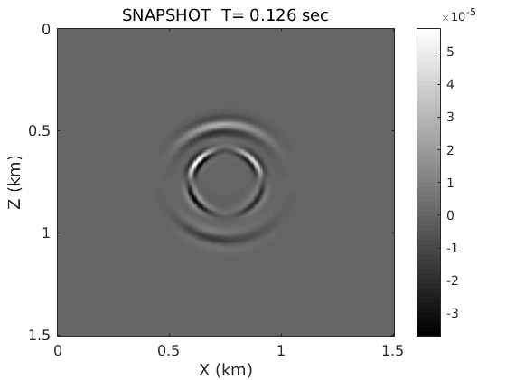
Viscoelastic modeling using staggrid finite difference method
fd_order=28;fsz=0;source_type='tau_zz';is=1;isfs=0;

% FD time loop and plot the snapshot of vertical partical velocity
staggerfd(nbc,nt,dtx,dx,dt,sx,sz,source,vp,vs,den,taup_epsilon,taus_epsilon,tausigma,isfs,fsz,fd_order,source_type);


Homework
1) Go through the code and run.