|
|
|
| Phase-Shift Migration Lab |
|
| This lab contains parameterizable code
for exploring phase-shift migration with thin lens and wide angle corrections. Three
input data sets are given, a band-limited impulse, a wide-band impulse, and a slice from the
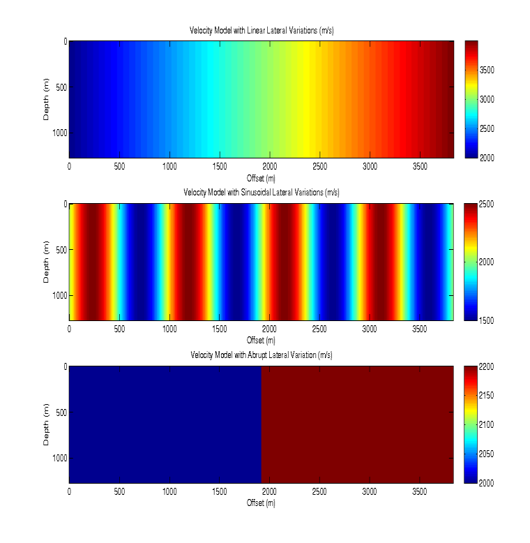
SEG/EAGE salt model. Three velocity models are given (pictured below) for use with in testing
the migration operator impulse responses. The input data set and velocity model are all
chosen by setting parameters at the top of run_psmig.m. You can also choose whether to include
thin lens and/or 15 degree and/or 45 degree wide anlge corrections by setting the appropriate
paramters. You can run a single migration with any combination of corrections or run a comparison
of four migrations progressively adding corrections by setting/unsetting the run_all parameter. You will need the following files data_band_limited.m, data.mat, data_wide_band.m, psmig.m, run_psmig.m, vel_lateral_abrupt.m", vel_lateral_linear.m, vel_lateral_sin.m, and vel.mat |
 |
|
1. Run a set of four comparison impulse responses using the band-limited data set with the linear velocity model. By setting the run_all parameter to 1, four iterations are run: 1. phase-shift only, 2. phase-shift with thin lens correction, 3. phase-shift with thin lens and 15 degree wide angle correction, and 4. phase-shift with thin lens, 15 and 45 degree wide angle corrections. Study the images produced and explain the effects of each correction step.
|
|
|
2. Repeat this step with the abrupt and sinusoidal velocity models. Do these models give you any further insight into the correction steps? Alter the velocity model parameters or create your own velocity models for further study.
|
|
|
3. Now change to the wide-band data set and experiment with different velocity models. You may want to set run_all to 0 and run a single migration with a combination of correction steps. Explain the artifacts in the image(s) produced. Why are they present? Study the construction of the band-limited and wide-band data sets and describe their differences.
|
|
|
4. Go back to the band-limited data set and choose a frequency band for migration from 10-35 Hz. How has the image changed and why? Find a minimal frequency band for migration which is not aliased. Why is this frequency band advantageous?
|
|
|
5. Study the migration code and describe the domain in which each of the operations takes place.
|
|
|
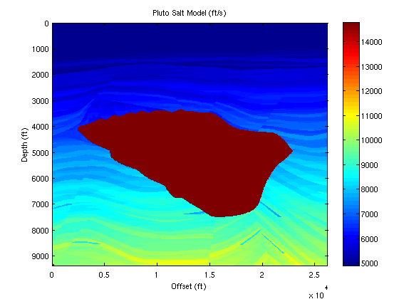
6. A zero-offset data set is provided for the SMAARTJV Pluto velocity model. Perform a series of migrations on this salt model with different combinations of correction techniques. Identify the effects of the wide angle corrections. Why are these important? Some erroneous strong reflections are present at depths well below the salt body. Explain the origins of these artifacts and how they could be avoided.
|
|
 |
|
| Written by Samuel Brown - Summer 2006 |