Theory

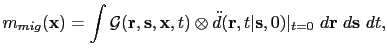
The theory for generalized diffraction-stack migration (GDM) was described by Schuster (2002), who reformulated the equations of RTM so that they can be reinterpreted as a GDM algorithm,

$$m_{mig}({\bf {x}}) =\int\mathcal G({\bf {r}},{\bf {s}},{\bf {x}}... ...mes \ddot{d}({\bf {r}},t\vert{\bf {s}},0)\vert _{t=0}~d{\bf {r}}~d{\bf {s}}~dt,$$ (17)

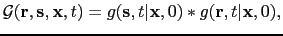
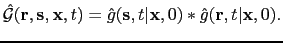
with the migration kernel defined as

$$\mathcal G({\bf {r}},{\bf {s}},{\bf {x}},t) = g({\bf {s}},t\vert{\bf {x}},0) \ast g({\bf {r}},t\vert{\bf {x}},0),$$ (18)

where $*$ denotes temporal convolution and $\otimes$ , together with $t=0$ , represents the correlation at zero-lag time (which is equivalent to a dot product in the data coordinates). The $\ddot{d}({\bf {r}},t\vert{\bf {s}},0)$ term represents the second time derivative of the trace at the receiver point ${\bf {r}}$ with the source point at ${\bf {s}}$ , while the $g({\bf {s}},t\vert{\bf {x}},0)$ and $g({\bf {r}},t\vert{\bf {x}},0)$ terms represent the scattered Green's functions which, respectively, propagate the energy from the subsurface trial image point ${\bf {x}}$ to the surface source point at ${\bf {s}}$ and the receiver point ${\bf {r}}$ . The term $\mathcal G({\bf {r}},{\bf {s}},{\bf {x}},t)$ acts as the migration operator or focusing kernel (Schuster, 2002) which migrates the reflection in $\ddot{d}({\bf {r}},t\vert{\bf {s}},0)$ to the trial image point ${\bf {x}}$ . It is obtained by a FD solution to the wave equation with a point source ${\bf {s}}$ on the surface and a scattering point at the image point ${\bf {x}}$ , and convolving this source-side Green's function $g({\bf {s}},t\vert{\bf {x}},0)$ with the receiver-side Green's function $g({\bf {r}},t\vert{\bf {x}},0)$ .

Figure: Diffraction-stack migration versus generalized diffraction-stack migration. a) Simple diffraction-stack migration operator (dashed hyperbola) and data, which only contains first arrival scattering information. b) Generalized diffraction-stack migration operator (dashed hyperbolas) which contains all events in the migration model, including multiples, diffractions and reflections.

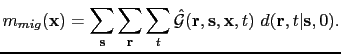
A simple diagram shown in Figure  illustrates the difference between the diffraction-stack migration and GDM operators plotted in data-space coordinates. Figure a shows the traditional migration curve for diffraction-stack migration which is also known as Kirchhoff migration. The usual interpretation is that the migration image at ${\bf {x}}$ is given by summing the trace amplitudes along the hyperbola, i.e., the migration image is the dot product of the recorded shot gathers with the migration operator (a single hyperbolic curve shown in Figure a). Figure b illustrates the idea behind GDM: take the dot product of the recorded shot gathers with the generalized migration operator $\mathcal G({\bf {r}},{\bf {s}},{\bf {x}},t)$ . Note that all events are included in the generalized migration operator such as direct waves, multiples, reflections and diffractions as well.

But the major problem with the above approach is that the migration operator $\mathcal G({\bf {r}},{\bf {s}},{\bf {x}},t)$ is a five-dimensional matrix with the dimension size determined by the model size, the number of sources and receivers, and the number of samples within a trace. It means that $\mathcal G({\bf {r}},{\bf {s}},{\bf {x}},t)$ is too expensive to be stored. To reduce the the cost of I/O and storage of the $\mathcal G({\bf {r}},{\bf {s}},{\bf {x}},t)$ , I only store the early-arrivals of $g({\bf {s}},t\vert{\bf {x}},0)$ followed by skeletonization to reduce the size of the migration kernel by at least two orders-of-magnitude.

The skeletonized least-squares GDM algorithm is as follows:

1. Compute the Green's functions $g({\bf {s}},t\vert{\bf {x}},0)$ by a numerical solution to the wave equation for a point source at trial image point ${\bf {x}}$ and recorded at source position ${\bf {s}}$ . Since ${\bf {s}}$ occupies the same positions as ${\bf {r}}$ , then $g({\bf {r}},t\vert{\bf {x}},0)$ is considered the same as $g({\bf {s}},t\vert{\bf {x}},0)$ .

2. Skeletonize $g({\bf {s}},t\vert{\bf {x}},0)$ to $\hat{g}({\bf {s}},t\vert{\bf {x}},0)$ . Early-arrivals are used and each important early-arrival event is replaced by a single time sample after skeletonization. In this way, a calculated Green's function trace with 501 samples is reduced to a sparse trace with about 25 samples.

3. The skeletonized Green's function $\hat{g}({\bf {s}},t\vert{\bf {x}},0)$ is associated with the recording position at ${\bf {s}}$ and $\hat{g}({\bf {r}},t\vert{\bf {x}},0)$ is that recorded at ${\bf {r}}$ . Those two Green's functions are convolved to generate the migration kernel:
   

   $$\hat{\mathcal G}({\bf {r}},{\bf {s}},{\bf {x}},t) =\hat{g}({\bf {s}},t\vert{\bf {x}},0) \ast \hat{g}({\bf {r}},t\vert{\bf {x}},0).$$ (19)

   
   

4. The migration operator $\hat{\mathcal G}({\bf {r}},{\bf {s}},{\bf {x}},t)$ is a Kirchhoff-like kernel that describes, for a single shot gather, pseudo-hyperbolas of multiarrivals in ${\bf {r}}-t$ space. The reflection energy in a recorded shot gather $d({\bf {r}}, t\vert{\bf {s}},0)$ is then summed along such pseudo-hyperbolas to give the migration image,
   

   $$m_{mig}({\bf {x}}) =\sum_{{\bf {s}}}\sum_{{\bf {r}}}\sum_{t}\hat{\mathcal G}({\bf {r}},{\bf {s}},{\bf {x}},t)~d({\bf {r}},t\vert{\bf {s}},0).$$ (20)

   
   

5. The above $\hat{\mathcal G}({\bf {r}},{\bf {s}},{\bf {x}},t)$ is used for iterative LSM by a conjugate gradient method.

The advantages of skeletonized least-squares GDM are that 1). the high-frequency approximation of Kirchhoff migration is largely not needed; 2). the storage requirement for the migration kernel is reduced by more than two orders-of-magnitude compared to storing every sample in a calculated migration kernel; 3). these migration operators do not need to be recalculated for each LSM iteration; 4). inclusion of just a few important early-arrival events can significantly reduce artifacts seen in conventional RTM images.

In contrast, the main drawback of skeletonized least-squares GDM is that the choice of important events is somewhat arbitrary and so can lead to missing important information in the migration operator. However, the migration operator is only as accurate as our knowledge of the subsurface velocity model so important events might be just the early-arrivals.