Least-squares Migration

For conventional least-squares migration (Nemeth et al., 1999), a reflectivity model $\textbf{m}$ is assumed to be independent of the shot position. For a dataset with $N_s$ shots, the modeling process can be expressed as

$$\begin{bmatrix} \textbf{d}_1\\ \textbf{d}_2\\ \cdot\\ \tex... ...L}_2 \\ \cdot\\ \textbf{L}_{N_s} \end{bmatrix}\left [ \textbf{m} \right ],$$ (24)

and similarly for the migration

$$\textbf{m}_{mig}=\left [ \textbf{L}^T_1~\textbf{L}^T_2~\cdot~\tex... ...\\ \textbf{d}_{N_s} \end{bmatrix}=\sum^{Ns}_{i=1}\textbf{L}^T_i\textbf{d}_i,$$ (25)

where the final image is the stack of migration images from all of the individual shots.

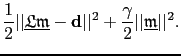
For conventional least-squares migration, a reflectivity model $\textbf{m}$ is sought that minimizes the misfit functional

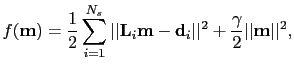$$f(\textbf{m})=\frac{1}{2}\sum^{N_s}_{i=1}\vert\vert\textbf{L}_i\t... ...m}-\textbf{d}_i\vert\vert^{2}+\frac{\gamma}{2}\vert\vert\textbf{m}\vert\vert^2,$$ (26)

where $\gamma$ is the damping coefficient, and $\textbf{m}$ is defined as the stacked migration image. This method will also be referred as least-squares migration with the stacked image. In Dai et al. (2012), the stacked migration image is computed from a blend of phase encoded shot gathers, also known as a supergather. When the migration velocity is not accurate, the prestack images are not exactly the same from different shots, and the stacked image can become blurred and convergence stalls.

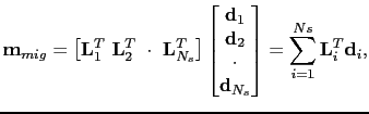
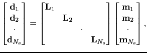
In order to improve the robustness of LSRTM, I define the ensemble of prestack images as a function of the shot position: $\underline{\mathfrak{m}} \rightarrow \underline{\mathfrak{m}}(\textbf{x},\textbf{x}_s)$ , or in matrix-vector notation

$$\underline{\mathfrak{m}}= \begin{bmatrix} \textbf{m}_1\\ \textbf{m}_2\\ \cdot\\ \textbf{m}_{N_s} \end{bmatrix},$$ (27)

where $\textbf{m}_i$ is the migration image for the $ith$ shot. Now for a dataset with $N_s$ shots, the forward modeling operation is

$$\begin{bmatrix} \textbf{d}_1\\ \textbf{d}_2\\ \cdot\\ \tex... ... \textbf{m}_1 \\ \textbf{m}_2 \\ \cdot\\ \textbf{m}_{N_s} \end{bmatrix},$$ (28)

and the migration operation is

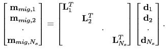$$\begin{bmatrix} \textbf{m}_{mig,1}\\ \textbf{m}_{mig,2}\\ \c... ... \textbf{d}_1 \\ \textbf{d}_2 \\ \cdot\\ \textbf{d}_{N_s} \end{bmatrix}.$$ (29)

For simplicity, I define $\underline{\mathfrak{L}}$ as the forward modeling operator for all the shot gathers

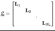$$\underline{\mathfrak{L}}= \begin{bmatrix} \textbf{L}_1 & & &\\ &\textbf{L}_2& & \\ & & \cdot&\\ & & & \textbf{L}_{N_s} \end{bmatrix}$$ (30)

and equation and are rewritten in compact form

$$\textbf{d}=\underline{\mathfrak{L}}\underline{\mathfrak{m}}$$ (31)

and

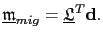$$\underline{\mathfrak{m}}_{mig}=\underline{\mathfrak{L}}^T\textbf{d}.$$ (32)

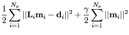
Therefore, the misfit functional with the ensemble of prestack images is defined as

$$f(\underline{\mathfrak{m}}) = \frac{1}{2}\sum^{N_s}_{i=1}\vert\vert\textbf{L}_i\textbf{m}_i-\te... ...ert\vert^{2}+\frac{\gamma}{2}\sum^{N_s}_{i=1}\vert\vert\textbf{m}_i\vert\vert^2$$

$$= \frac{1}{2}\vert\vert\underline{\mathfrak{L}\mathfrak{m}}-\textbf{d}\vert\vert^{2}+\frac{\gamma}{2}\vert\vert\underline{\mathfrak{m}}\vert\vert^2.$$ (33)

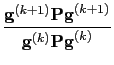
A preconditioned conjugate gradient algorithm

$$\textbf{g}^{(k+1)} = \underline{\mathfrak{L}}^{T}[\underline{\mathfrak{L}\mathfrak{m}}^{(k)}-\textbf{d}]+\gamma \underline{\mathfrak{m}}^{(k)}$$

$$\beta = \frac{\textbf{g}^{(k+1)}\textbf{Pg}^{(k+1)}}{\textbf{g}^{(k)}\textbf{Pg}^{(k)}}$$

$$\textbf{z}^{(k+1)} = \textbf{Pg}^{(k+1)}+\beta \textbf{z}^{(k)}$$

$$\alpha = \frac{[\textbf{z}^{(k+1)}]^{T}\textbf{g}^{(k+1)}}{[\textbf{Lz}^{(k+1)}]^{T}\textbf{Lz}^{(k+1)}+\lambda \vert\vert\textbf{z}^{(k+1)}\vert\vert^2}$$

$$\underline{\mathfrak{m}}^{(k+1)} = \underline{\mathfrak{m}}^{(k)}-\alpha \textbf{z}^{(k+1)},$$ (34)

can be implemented to find the solution $\underline{\mathfrak{m}}$ that minimizes the misfit in equation . In above equation, $\textbf{P}$ is the matrix representing the illumination compensation preconditioner (Plessix and Mulder, 2004).

The ensemble of prestack images $\underline{\mathfrak{m}}$ contains many more unknowns than the stacked image, and therefore provides more freedom to fit the observed data (see Appendix C). Another advantage is that the common image gathers can be extracted from the prestack images as an indication of the image quality.