


Next: Numerical results
Up: Theory
Previous: Least-squares Migration
Contents
In Dai et al. (2012), the multisource technique is implemented with random time shifts and random source polarity encoding functions to greatly reduce the computational cost. By stacking images from different supergathers and gradients from different iterations, the coherent signal is enhanced while the crosstalk noise is reduced.
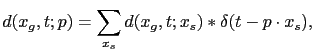
In this report, the shot-domain data are encoded with linear time-shift encoding functions and transformed into plane waves. Assuming a 2D survey geometry, the encoding process can be expressed as:
 |
(35) |
where the shot-domain data
 are encoded with a time shift function
 and stacked together. As illustrated by Figure
 ![[*]](file:~/utilities/latex2html/icons/crossref.png) , the time shift
, the time shift
 is a linear function of source position
  , and
, and  is the ray parameter defined as
 |
(36) |
where  is the surface shooting angle and
  is the velocity at the surface. For the 3D case, the plane-wave is computed from linear combination of surface sources along the
  -direction or both the
- and
-direction or both the
- and  -directions to form planar sources (see Zhang et al. (2005) and Duquet Lailly (2006) for details).
Since the plane waves are coherent signals, the migration image of one plane wave does not contain crosstalk noise seen in the migration image of a phase-encoded supergather. Instead, it contains aliasing artifacts, which can be reduced by stacking images from many different angles. Zhang et al. (2005) provided an estimate of how many angles are needed as a function of recording aperture, velocity model, and estimated dipping angle range of the reflectors.
-directions to form planar sources (see Zhang et al. (2005) and Duquet Lailly (2006) for details).
Since the plane waves are coherent signals, the migration image of one plane wave does not contain crosstalk noise seen in the migration image of a phase-encoded supergather. Instead, it contains aliasing artifacts, which can be reduced by stacking images from many different angles. Zhang et al. (2005) provided an estimate of how many angles are needed as a function of recording aperture, velocity model, and estimated dipping angle range of the reflectors.
Figure:
The diagram of plane wave encoding (reproduced from Zhang et al. (2005)), where the time shift is linear function to the source location
and the slope is the ray parameter
.
|
|
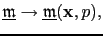
In the plane-wave domain, the prestack image ensemble is a function of the ray parameter
 |
(37) |
or in matrix-vector notation
 |
(38) |
assuming there are  plane-wave gathers. In above equation,
 is the image associated with the
  plane-wave gather.
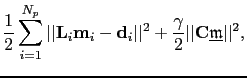
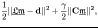
A new misfit functional is defined in the plane-wave domain as
plane-wave gather.
A new misfit functional is defined in the plane-wave domain as
Note that
 represents the
plane-wave gather and
represents the
plane-wave gather and
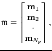
 is the forward modeling operator associated with it. In this chapter, I choose a regularization term that penalizes the difference of migration images computed with slightly different incidence angles, and it is defined as
 |
(40) |
 is the damping coefficient and is chosen empirically.
Then a preconditioned conjugate gradient scheme similar to equation can be implemented:
is the damping coefficient and is chosen empirically.
Then a preconditioned conjugate gradient scheme similar to equation can be implemented:
to find the LSRTM prestack images. In the next section, unless otherwise denoted, all LSRTM images are produced with the proposed new method.
Next: Numerical results
Up: Theory
Previous: Least-squares Migration
Contents
Wei Dai
2013-07-10
![\includegraphics[width=4.0in]{./chap3.plane.img/plane_shoot.eps}](img141.png)
![$\displaystyle \frac{[\textbf{z}^{(k+1)}]^{T}\textbf{g}^{(k+1)}}{[\textbf{Lz}^{(k+1)}]^{T}\textbf{Lz}^{(k+1)}+\lambda \vert\vert\textbf{Cz}^{(k+1)}\vert\vert^2}$](img149.png)