Deblurring filter

Following Aoki and Schuster (2009), I use a grid model with an even distribution of isolated point scatterers $\textbf{m}_{ref}$ as my reference model. According to equation (6), I get

$$\textbf{m}_{mig\_ref}=\textbf{L}^{T}\textbf{Lm}_{ref}=\textbf{L}^{T}\textbf{d},$$ (65)

where $\textbf{L}$ is the linear diffraction stack operator, which only depends on the background velocity $\textbf{v}_{o}$ and the source receiver configurations. Here a column of the $\textbf{L}^{T}\textbf{L}$ matrix represents a migration Green's function (Schuster and Hu, 2000). Then, as shown in Figure A.1 I divide $\textbf{m}_{ref}$ into somewhat large subsections centered around each point scatterer. In each subsection, I define a small-sized filter $\textbf{f}_{i}$ , such that

$$\textbf{[m}_{mig\_ref}\textbf{]}_{i}*\textbf{f}_{i}=\textbf{[m}_{ref}\textbf{]}_{i}.$$ (66)

where $i$ indicates the ith subsection and the notation $\textbf{[ ]}_{i}$ denotes the model in the ith subsection. It is very important to choose a proper size for $\textbf{[m}_{ref}\textbf{]}_{i}$ as it has to be big enough to cover the main part of the migration butterflies (Schuster and Hu, 2000). In each sub-section, the reference model $\textbf{[m}_{ref}\textbf{]}_{i}$ only contains a point scatterer. Thus, $\textbf{[m}_{mig\_ref}\textbf{]}_{i}$ represents a migration Green's function, but truncated by the sub-section and $\textbf{f}_{i}$ is a local filter, which approximates the inverse of the Hessian within the sub-section. After solving for $\textbf{f}_{i}$ by a least-squares method, I apply $\textbf{f}_{i}$ to the ith subsection of the original migration image obtained from the field data, and construct another image $\textbf{m}_{mf}$ . Near the boundaries between sub-sections, linear interpolation of nearby local filters is computed to make a smoothly varying image. This process can be expressed as

$$\textbf{m}_{mf}=\textbf{m}_{mig}*\textbf{f}.$$ (67)

Here, $\textbf{f}$ represents a bank of stationary filters (each filter is constant within its corresponding subsection). We can rewrite equation A.3 in matrix notation

$$\textbf{m}_{mf}=\textbf{Fm}_{mig}.$$ (68)

Since $\textbf{m}_{mf}$ is an approximation of $\textbf{m}$ , and

$$\textbf{m}=\textbf{(L}^{T}\textbf{L)}^{-1}\textbf{m}_{mig},$$ (69)

then the computed $\textbf{f}_{i}$ in each subsection can be formed as the approximated preconditioner matrix

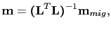
Figure A.1: Steps for computing the deblurring filter. Step (a) Define smooth velocity model with point scatterers denoted as circles in (b). Generate multisource data in (c), migrate the multisource data and get an image shown in (d). Step (e), in each sub-section, compute a local filter according to $\textbf {[m}_{mig\_ref}\textbf {]}_{i}*\textbf {f}_{i}=\textbf {[m}_{ref}\textbf {]}_{i}$ and combine all the local filters into the deblurring filter $\textbf {F}$ .

$$\textbf{F}\approx\textbf{(L}^{T}\textbf{L)}^{-1}.$$ (70)

We can improve the standard migration image by applying $\textbf {F}$ to it, or, I can use $\textbf {F}$ as a preconditioner in an iterative LSM solution to speed up convergence.

There are limitations associated with the deblurring filter.

1. The sub-section needs to be big enough to cover the main part of migration artifacts. It also has to be large in order to avoid the interface between neighboring sections.

2. The migration Green's function is constant within a sub-section, so that I can keep the filter constant with the sub-section. To honor these two approximations, the velocity model needs to be smooth, so that the variation in the migration Green's function is smooth; hence, I usually use a high-frequency Ricker source wavelet, which makes the migration artifacts smaller.