


Next: Numerical Scheme: Quasi-linear Inversion
Up: Theory
Previous: Theory
Contents
Given a background slowness model
 , the Green's function for the Helmholtz equation is the solution of
![$\displaystyle [\bigtriangledown^{2}+\omega^{2} \textbf{s}_{o}(\textbf{x})^{2}] G_{o}(\textbf{x}\vert\textbf{x}_{s})= -\delta(\textbf{x}-\textbf{x}_{s}),$](img21.png) |
(21) |
where
 is the Green's function associated with the background slowness
and an impulsive point source at
is the Green's function associated with the background slowness
and an impulsive point source at
 ,
,
 is the listening location, and
  is the angular frequency. For a point source at
with spectrum
is the angular frequency. For a point source at
with spectrum  (corresponding to the source term
 ), the solution is
 .
.
If the background slowness perturbation is represented by the amount of
 , the true slowness model is described by
 . The full wavefield is obtained by solving the Helmholtz equation with slowness model
 ,
,
![$\displaystyle [\bigtriangledown^{2}+\omega^{2} \textbf{s}(\textbf{x})^{2}]\textbf{P}=F,$](img32.png) |
(22) |
with the same source term
 as before.
Our goal is to calculate the scattered wavefield
as before.
Our goal is to calculate the scattered wavefield
 induced by the slowness perturbation
with a linear modeling operator. Plugging
into equation (2.2), I get
induced by the slowness perturbation
with a linear modeling operator. Plugging
into equation (2.2), I get
![$\displaystyle [\bigtriangledown^{2}+\omega^{2} \textbf{s}_{o}(\textbf{x})^{2}+2\omega^{2} \textbf{s}_{o}(\textbf{x})\delta \textbf{s}(\textbf{x})] \textbf{P}= F,$](img35.png) |
(23) |
where the high order term
 is neglected. According to Green's theorem, moving the 3rd term in equation (2.3) to the right side, multiplying both sides with the Green's function
 and integrating over the whole volume with index
 , gives the Lippmann-Schwinger equation,
which is an integral equation with unknown
 on both sides and
 representing the reflectivity model. Here,
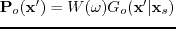
 is the pressure field associated with the background velocity model. Defining
 and applying the Born approximation
 to the right side and assuming that
is small gives the scattered field under Born approximation
to the right side and assuming that
is small gives the scattered field under Born approximation
where formula (2.5) represents a non-linear equation for calculation of the scattered wavefield and equation (2.6) is a linear equation (Mulder and Plessix, 2004a).
With
 , the linear modeling requires the solutions of
![$\displaystyle [\bigtriangledown^{2}+\omega^{2}\textbf{s}_{o}(\textbf{x})^{2}]\textbf{P}_{1}= \omega^2 \textbf{m}(\textbf{x}')\textbf{P}_{o}(\textbf{x}').$](img54.png) |
(27) |
These fields can be computed by two finite-difference simulations: one with the original point source  and background slowness model
to generate
and background slowness model
to generate
 ; The second finite-difference simulation also uses the background slowness model
, but the source term is
; The second finite-difference simulation also uses the background slowness model
, but the source term is
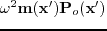 , where
 becomes the 2nd-order time derivative in the time domain.
The adjoint of the linear operator is the reverse time migration (RTM) operator, so the RTM equation is
becomes the 2nd-order time derivative in the time domain.
The adjoint of the linear operator is the reverse time migration (RTM) operator, so the RTM equation is
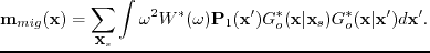 |
(28) |
In the following section, matrix-vector notation will be used to represent the operators, such that the non-linear modeling operator is defined as
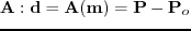 , the linear modeling operator is
 , and the reverse time migration operator is
 . The modeling operator
 is called the Fréchet derivative of
 and
and
 is the adjoint of
.
is the adjoint of
.
Next: Numerical Scheme: Quasi-linear Inversion
Up: Theory
Previous: Theory
Contents
Wei Dai
2013-07-10