Signal-to-Noise Analysis

If a higher SNR is demanded, more iterations should be used. Alternatively, the input data should consist of a number of sub-supergathers rather than one comprehensive supergather that contains all the shot records. Any sub-supergather should contain a distinct blend of encoded shot gathers. The benefit is an enhancement of the SNR but the cost is an extra RTM simulation for each sub-supergather. Schuster et al. (2011) and Dai et al. (2011) have shown that the SNR of the stacked migration images after phase encoding is proportional to the square root of the number of supergathers ($N$ ) used for the migration,

$$\textrm{SNR} \propto \sqrt{NI},$$ (213)

where $I$ indicates the number of stacks by an iterative stacking method. The SNR of the LSRTM image is expected to approximately behave in a similar manner.

To verify the prediction from equation (2.13), the LSRTM algorithm is applied to four and eight supergathers to produce images in Figure 2.4(c) and 2.4(d), respectively, after 30 iterations. All the images in Figure 2.4 are filtered with the same high-pass filter. By examining the gradual change from Figure 2.4(b) to (d), it is clear that increasing the number of supergathers greatly improves the quality of the LSRTM images and the numerical tests largely agree with the prediction from equation (2.13).

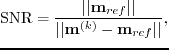
To measure how the SNR of the multisource LSRTM image is changing with the number of iterations, the total number of shots is reduced to 300 so that I can afford to carry out LSRTM with conventional single source data. Then, all 300 shots are encoded together in one supergather for multisource LSRTM. Numerically, I use the formula

$$\textrm{SNR}=\frac{\vert\vert\textbf{m}_{ref}\vert\vert}{\vert\vert\textbf{m}^{(k)}-\textbf{m}_{ref}\vert\vert},$$ (214)

to calculate the SNR at each iteration, where the conventional sources LSRTM image at the same iteration is used as the reference signal. The assumption is that the convergence rates for multisource and conventional sources LSRTM are the same. Figure 2.5 shows that the convergence curves for the two experiments are similar, which suggests the validity of the above assumption. Figure 2.6 shows (a) the LSRTM image at the 1st iteration for conventional sources data after high-pass filtering, (b) the 1st iteration LSRTM image for one 300-shot supergather after high-pass filtering, and (c) the difference between the above images before filtering. Since the crosstalk noise in the shallow part of the image is masked by back-scattering migration artifacts, only the part of the image below 6 km is used for SNR calculation.

Figure 2.7 shows the measured SNR as a function of the number of iterations. The measurements are normalized by the 1st iteration result and compared to the prediction from equation 2.13. In Figure 2.7 the measurements in general are slightly below the prediction. As explained by Dai et al. (2011), when the LSRTM image is viewed as a weighted summation of the gradients from each iteration, early iterations generally receive large weights because of the large data residual associated with them. In term of reducing random crosstalk noise, the weighted summation is less effective than direct summation.