


Next: Prism Wave Reverse Time
Up: Reverse Time Migration of
Previous: Introduction
Contents
In the frequency domain, reverse time migration of a shot gather
 can be expressed as
 |
(42) |
where
 is the migration image of the shot at
 ,
,
 is the source spectrum,
 indicates the receiver location,
 is the Green's function from a source at
to
is the Green's function from a source at
to
 ; This Green's function is computed by a finite-difference solution to the wave equation. The
  indicates complex conjugate. For simplicity, the angular frequency
  is silent in the Green's function
  and data function
  .
.
For the velocity model in Figure ![[*]](file:~/utilities/latex2html/icons/crossref.png) (a), referred to as the L model, the recorded data contain prism waves. The yellow arrows in Figure (a) indicate the ray path for a prism wave excited at
(a), referred to as the L model, the recorded data contain prism waves. The yellow arrows in Figure (a) indicate the ray path for a prism wave excited at
 and recorded at
 , and Figure (b) depicts the wavepath (Luo and Schuster, 1991) of the prism wave generated by a source with a 20-Hz Ricker wavelet.
The recorded trace is plotted in Figure (c) with a red window outlining the reflection from the horizontal reflector and the prism wave. For simplicity, I mute the direct wave and diffractions from the trace to keep only the part in the red window
, and Figure (b) depicts the wavepath (Luo and Schuster, 1991) of the prism wave generated by a source with a 20-Hz Ricker wavelet.
The recorded trace is plotted in Figure (c) with a red window outlining the reflection from the horizontal reflector and the prism wave. For simplicity, I mute the direct wave and diffractions from the trace to keep only the part in the red window
 |
(43) |
where
 and
and
 denote the first-order scattering reflection wave and the doubly scattered prism wave, respectively.
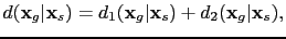
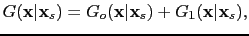
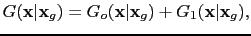
When the horizontal reflector is extracted from the migration images and embedded in the migration velocity model (Figure (a)), conventional RTM can correctly migrate the prism waves to image the vertical reflector (Jones et al., 2007). In this case, the Green's function calculated with the migration velocity in Figure (a) contains two arrivals: a direct wave arrival and a reflection from the horizontal reflector as shown in Figure . Therefore, the Green's functions in equation can be decomposed into two parts:
denote the first-order scattering reflection wave and the doubly scattered prism wave, respectively.
When the horizontal reflector is extracted from the migration images and embedded in the migration velocity model (Figure (a)), conventional RTM can correctly migrate the prism waves to image the vertical reflector (Jones et al., 2007). In this case, the Green's function calculated with the migration velocity in Figure (a) contains two arrivals: a direct wave arrival and a reflection from the horizontal reflector as shown in Figure . Therefore, the Green's functions in equation can be decomposed into two parts:
 |
(44) |
and
 |
(45) |
where  and
and  denote the direct and the reflected waves, respectively. Note that in this case
is a downgoing wave and
is an upgoing wave.
denote the direct and the reflected waves, respectively. Note that in this case
is a downgoing wave and
is an upgoing wave.
Figure 4.2:
(a) A two-layer velocity model. The star and triangle indicate the source and receiver locations. The yellow arrow is the ray path for the direct wave and the red arrows show the ray path for the reflected wave. (b) The trace recorded at the triangle. It is simulated with a 20-Hz Ricker wavelet.
|
|
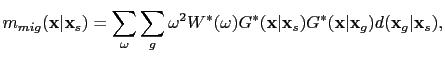
When the data in the red window of Figure (c) are migrated with the velocity model in Figure (a), the migration image is shown in Figure (b), and is mathematically described by
| |
|
 |
|
| |
 |
![$\displaystyle \sum_{\omega}\omega^2 {W}^* (\omega) [{G}_o^* (\textbf{x}\vert\te...
...)][{d}_1 (\textbf{x}_g\vert\textbf{x}_s)+{d}_2 (\textbf{x}_g\vert\textbf{x}_s)]$](img202.png) |
|
| |
|
 |
(46) |
| |
 |
 |
(47) |
| |
|
 |
(48) |
| |
|
 |
(49) |
| |
|
 |
(50) |
| |
|
 |
(51) |
| |
|
 |
(52) |
Note that the summation over the receiver  is omitted because there is only one trace in this example.
With the assumption that the reflection coefficient is the angle-independent value
is omitted because there is only one trace in this example.
With the assumption that the reflection coefficient is the angle-independent value  , the amplitude of the direct wave Green's function
  is on the order of
  and the amplitude of the reflection wave
  is on the order of
  . Similarly,
  is with strength of
. The prism wave
is with strength of
. The prism wave  is a doubly scattered wave and its amplitude is on the order
  .
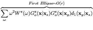
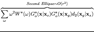
As an example, the first prism wave term in equation has
.
As an example, the first prism wave term in equation has  because it is a product of the
term with amplitude
and the migration kernel
because it is a product of the
term with amplitude
and the migration kernel
 with strength
.
With these assumptions, the amplitude of each term in the above equation can be expressed in terms of
as shown in the labels.
with strength
.
With these assumptions, the amplitude of each term in the above equation can be expressed in terms of
as shown in the labels.
Figure:
(a) The homogeneous velocity ( ) with a horizontal reflector embedded (
 ); (b) the migration image of the data within the red window in Figure 4.1(a) with the velocity model in panel (a).
|
|
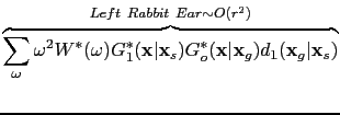
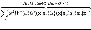
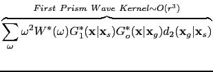
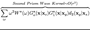
Figure (b) shows two ellipses. The first one corresponds to the migration kernel in equation with the strongest amplitude
. When the prism wave is migrated as a primary wave (the term in equation ), it shows up as the second ellipse in Figure (b) with an amplitude
. This ellipse is an artifact. The migration kernels in equations and correspond to these two ``rabbit ears'' with the strength
. Equations and contain the migration kernels for the prism waves corresponding to these near-vertical curves in Figure (b) and their amplitudes are on the order of
, which are much weaker than other kernels, so in the migration image, the vertical reflector is of weaker amplitude compared to the horizontal ones.
Subsections
Next: Prism Wave Reverse Time
Up: Reverse Time Migration of
Previous: Introduction
Contents
Wei Dai
2013-07-10
![\includegraphics[width=5.0in]{./chap4.prism.img/layers_greens.eps}](img200.png)
![\includegraphics[width=5.0in]{./chap4.prism.img/prism_kernel.eps}](img224.png)