


Next: Geometric Interpretation of the
Up: Theory
Previous: Theory
Contents
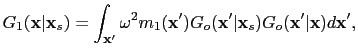
If the migration kernels in equations ![[*]](file:~/utilities/latex2html/icons/crossref.png) and can be computed directly, the prism waves can be directly migrated without crosstalk interference. In the following section, frequency domain formulas are used for mathematical simplicity, but the numerical calculation is actually computed in the time domain by a finite-difference solution to the space-time acoustic wave equation. Given a smooth migration velocity (homogeneous velocity in this example) and a migration image of the horizontal reflector, the Green's function for the reflected wave can be computed with the Born approximation (Stolt and Benson, 1986)
and can be computed directly, the prism waves can be directly migrated without crosstalk interference. In the following section, frequency domain formulas are used for mathematical simplicity, but the numerical calculation is actually computed in the time domain by a finite-difference solution to the space-time acoustic wave equation. Given a smooth migration velocity (homogeneous velocity in this example) and a migration image of the horizontal reflector, the Green's function for the reflected wave can be computed with the Born approximation (Stolt and Benson, 1986)
 |
(53) |
where
 is the reflectivity model representing the horizontal reflector, and the Green's function
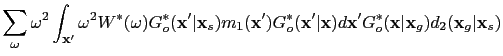
  is calculated using the migration velocity. Plugging equation into equation , I get
with
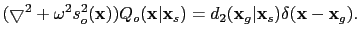
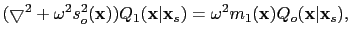
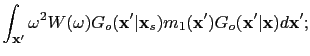
Numerically,
 are computed with two finite-difference simulations in the time domain to solve the following two equations
where the slowness
 is the reciprocal of the migration velocity model.
The receiver-side wavefield
is the reciprocal of the migration velocity model.
The receiver-side wavefield
 can be computed by solving
 |
(58) |
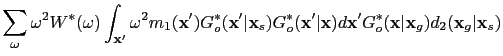
Note the wavefield propagates backward in time when solving the above equation in the time domain with the finite-difference method. When there is more than one trace in the shot gather, all the traces act as source wavelets of point sources at their respective recording locations, which implies a summation over the receiver  . In summary, prism wave migration requires three finite-difference simulations (equations , , and ) to calculate the image corresponding to the term in equation .
Figure illustrates the process of prism wave migration with equation : (1) The source wavefield
 propagates downward starting from the source location; (2)
is reflected at the horizontal reflector and becomes the reflected wavefield
propagates downward starting from the source location; (2)
is reflected at the horizontal reflector and becomes the reflected wavefield
 ; (3) The receiver wavefield
 propagates downward from the receiver; (4) The product of
and
is the migration image (the vertical curve in Figure is part of the prism wave migration kernel and computed by equation ).
propagates downward from the receiver; (4) The product of
and
is the migration image (the vertical curve in Figure is part of the prism wave migration kernel and computed by equation ).
Figure 4.4:
Diagrams of the ray paths illuminating the process of prism wave migration: (a) source and receiver wavefields correlate at the correct image point. Panels (b) and (c) show the ray paths to two image points that are above and below the right location. The black vertical curve plots part of the prism wave migration kernel. The circles along the curve show the locations of trial image points.
|
|
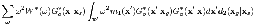
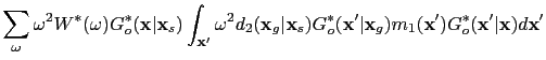
Similarly, the term in equation can be computed by
with
 computed by a finite-difference solution to
 |
(60) |
using the time reversed traces as source wavelets in equation .
Therefore, the migration image of the prism wave is the sum of the two terms from equations and ,
![$\displaystyle {m}_{mig}(\textbf{x}\vert\textbf{x}_s)=\omega^2 [{P}_1(\textbf{x}...
...2 [{P}_o(\textbf{x}\vert\textbf{x}_s)]^* [{Q}_1 (\textbf{x}\vert\textbf{x}_s)],$](img252.png) |
(61) |
and it requires four finite-difference simulations in total. Compared to conventional RTM, its computational cost is doubled. The advantages of this approach are as follows: (1) It avoids modifying the migration velocity as in conventional RTM of prism waves; (2) vertical structures are imaged in a separate step and reduces the crosstalk interference between different phases.
Next: Geometric Interpretation of the
Up: Theory
Previous: Theory
Contents
Wei Dai
2013-07-10
![\includegraphics[width=5.0in]{./chap4.prism.img/prism_path2.eps}](img246.png)
![$\displaystyle \sum_{\omega}\omega^2 [P_1(\textbf{x}\vert\textbf{x}_s)]^* [Q_o(\textbf{x}\vert\textbf{x}_s)],$](img230.png)
![$\displaystyle \sum_{\omega}\omega^2 [{P}_o(\textbf{x}\vert\textbf{x}_s)]^* [{Q}_1 (\textbf{x}\vert\textbf{x}_s)],$](img249.png)