Geometric Interpretation of the Migration Kernel for Prism Wave

When the migration velocity is a homogeneous model with velocity $c=~2~km/s$ , the reverse time migration kernel plots as an ellipse for fixed source and receiver locations, where the ellipse is defined by the formula

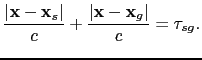$$\frac{\vert\textbf{x}-\textbf{x}_s\vert}{c}+\frac{\vert\textbf{x}-\textbf{x}_g\vert}{c}=\tau_{sg}.$$ (62)

Here $\tau_{sg}$ represents the travel time of a reflection arrival from the source at $\textbf{x}_s$ to the receiver at $\textbf{x}_g$ . If a prism wave reflects off the horizontal reflector first and then reflects from the vertical reflector (Figure (a)), and the depth of the horizontal reflector is known as $z_h$ , the migration traveltime equation corresponding to this prism wave can be defined as

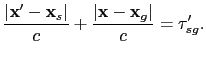$$\frac{\vert\textbf{x}'-\textbf{x}_s\vert}{c}+\frac{\vert\textbf{x}-\textbf{x}_g\vert}{c}=\tau_{sg}'.$$ (63)

In the above equation, $\tau_{sg}'$ is the travel time of the prism wave from $\textbf{x}_s$ to $\textbf{x}_g$ . For $\textbf{x}=(x,z)$ above the horizontal reflector, 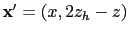$\textbf{x}'=(x,2z_h-z)$ is the mirror image of $\textbf{x}$ with respect to the horizontal reflector. For any $\textbf{x}$ below the horizontal reflector, according to Huygens principle, the Green's function ${G}_1(\textbf{x}\vert\textbf{x}_s)$ has an arrival time similar to that of the direct wave ${G}_o(\textbf{x}\vert\textbf{x}_s)$ , with an additional amplification caused by $\omega^2$ in equation . Therefore, below the horizontal reflector, the migration kernel plots as the ellipse in model space defined by

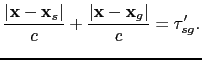$$\frac{\vert\textbf{x}-\textbf{x}_s\vert}{c}+\frac{\vert\textbf{x}-\textbf{x}_g\vert}{c}=\tau_{sg}'.$$ (64)

This ellipse is an artifact and can be removed by up-down dip filtering applied to the traces associated with $G_1$ (Zhan and Schuster, 2012).

Figure (a) depicts the migration kernel corresponding to the ray path in Figure (a) and equation . Figure (b) plots the curves defined by equations and , which are in excellent agreement with those associated with the migration kernel in Figure (a). In fact, equation illustrates the basis of Kirchhoff migration of prism waves (Marmalyevskyy et al., 2005). Similarly, the migration kernel of equation is plotted in Figure (b), which corresponds to the ray path in Figure (a). By symmetry considerations, it is obvious that a vertical reflector placed on the right side can also fit the observed prism wave. This kernel is plotted in Figure (c).

Figure 4.5: (a) The migration kernel of the prism wave corresponding to the term in equation 4.9 in the case the vertical reflector is on the left side. (b) The outline of the migration kernel in panel (a) according to the geometric interpretation. The star and triangle indicate the source and receiver locations respectively.

Figure 4.6: (a) The ray path for the prism wave with a vertical reflector on the right side; (b) the migration kernel of the prism wave corresponding to the term in equation 4.10 in the case the vertical reflector is on the right side; and (c) the outline of the migration kernel in panel (b) according to the geometric interpretation. The star and triangle indicate the source and receiver location respectively.