Least-squares Migration with Prestack Image

In least-squares migration, the goal is to solve the over-determined system of equations

$$\textbf{d}=\textbf{L}\textbf{m},$$ (77)

where $\textbf{d}$ is the data vector, $\textbf{L}$ matrix represents the forward modeling operator, and $\textbf{m}$ is the model vector, and the corresponding normal equation is

$$\textbf{L}^{T}\textbf{d}=\textbf{L}^{T}\textbf{L}\textbf{m}.$$ (78)

The direct least-squares solution is

$$\textbf{m}=[\textbf{L}^T\textbf{L}]^{-1}\textbf{L}^T\textbf{d}.$$ (79)

Assuming a dataset with three shots, each of dimension $N_g \times N_t$ , the total length of the data vector is $3N_g \times N_s$ . If the model vector is of the size $N_x \times N_z$ , the dimension of equation C.1 will be

$$\left [ \textbf{d} \right ]^{3N_{g}N_{s}}=\left [ \textbf{L}\right ]^{3N_{g}N_{s} \times N_{x}N_{z}} \left [ \textbf{m} \right ]^{N_{x}N_{z}}.$$ (80)

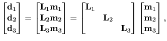
For example, if the three shots are $\textbf{d}_1$ , $\textbf{d}_2$ , and $\textbf{d}_3$ , each with the length of $N_g \times N_t$ , the above equation can be rewritten as

$$\begin{bmatrix} \textbf{d}_1\\ \textbf{d}_2\\ \textbf{d}_3 ... ...\\ \textbf{L}_2 \\ \textbf{L}_3 \end{bmatrix}\left [ \textbf{m} \right ],$$ (81)

where $\textbf{L}_1$ , $\textbf{L}_2$ , and $\textbf{L}_3$ are the forward modeling operator associated with each shot respectively. Here, $\textbf{d}_i$ denotes the shot gather for the $ith$ shot.

When the least-squares migration is performed with a stacked image as shown in equation C.5, the answer $\textbf{m}$ in equation C.3 is the solution to the whole problem. In this dissertation, I propose to introduce an ensemble of prestack images

$$\underline{\mathfrak{m}}=\begin{bmatrix} \textbf{m}_1\\ \textbf{m}_2\\ \textbf{m}_3 \end{bmatrix}$$ (82)

into the inversion scheme, so that the system of equations becomes

$$\begin{bmatrix} \textbf{d}_1\\ \textbf{d}_2\\ \textbf{d}_3 ... ...\begin{bmatrix} \textbf{m}_1\\ \textbf{m}_2\\ \textbf{m}_3 \end{bmatrix},$$ (83)

where $\textbf{m}_1$ , $\textbf{m}_2$ , and $\textbf{m}_3$ are the migration image associated for each shot respectively, each with the size of $N_x \times N_z$ . The direct solution to the equation C.7 is

$$\begin{bmatrix} \textbf{m}_1\\ \textbf{m}_2\\ \textbf{m}_3 \end... ...\ [\textbf{L}^T_3\textbf{L}_3]^{-1}\textbf{L}^T_{3}\textbf{d}_3 \end{bmatrix}.$$ (84)

It is clear that the solution $\textbf{m}_1$ , $\textbf{m}_2$ , and $\textbf{m}_3$ are independent of each other. By introducing the prestack image into the inversion, I solve three small problems instead of one big problem, thus make it possible to find stable solution when the equations are not consistent with each other in the case of wrong migration velocity.