Next: Bibliography
Up: Multisource Least-squares Migration and
Previous: Least-squares Migration with Prestack
Contents
Mathematical Derivation with Adjoint State Method
In Chapter 4, the physical meaning of prism wave migration was explained with a simple geometrical interpretation. From the mathematical point of view, the migration of prism waves can be thought of as the adjoint operation of modeling a prism wave. To show this, I will derive the forward modeling operator of a prism wave and apply the adjoint state method to derive its corresponding migration operator. Given a background slowness model
 and a reflectivity model
 , the reflection data for a shot at
 can be modeled with the Born approximation using the following equations (Dai et al., 2012)
By introducing a perturbation to the slowness model
 , the wavefields become
 ,
,
 . Expanding the slowness term as
 |
(87) |
equations D.1 and D.2 become
Assuming
 , and subtracting equation D.1 from equation D.4, I get
 |
(90) |
Similarly, subtracting equation D.2 from equation D.5, I get
 |
(91) |
where the higher order terms are neglected. Equation D.7 represents the modeling operator for the prism wave
 , which requires solving equations D.1, D.2, and D.6. Calculation of the prism wave needs four finite-difference simulations.
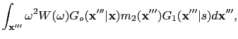
The above equations can be expressed with Green's functions  calculated with the slowness
  , so equation D.2 becomes
 |
(92) |
and equation D.6 becomes
 |
(93) |
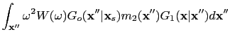
where
 and
and
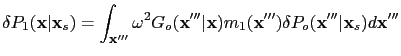
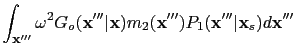
 are dummy variables. Thus, the modeling operator of the doubly scattered prism wave can be expressed as
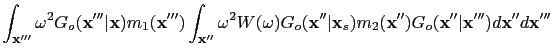
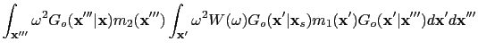
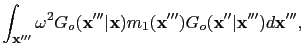
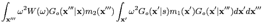
If I switch the order of integration for the first term, the above equation becomes
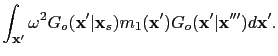
where  represents the Green's function for reflection wave:
When the wavefield
 is recorded at the receiver location
 , the shot gather
 of the prism wave can be expressed as
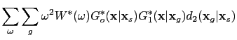
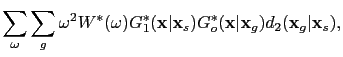
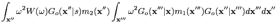
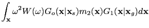
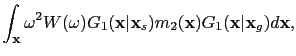
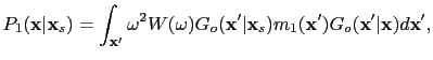
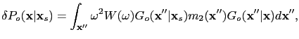
Equation D.14 is the forward modeling operator for the prism wave. By simply applying adjoint of the forward modeling (Plessix, 2006), the migration image of the shot gather
can be shown to be
which are exactly the terms in equations ![[*]](file:~/utilities/latex2html/icons/crossref.png) and . The computation of these terms is described in the text.
and . The computation of these terms is described in the text.
Next: Bibliography
Up: Multisource Least-squares Migration and
Previous: Least-squares Migration with Prestack
Contents
Wei Dai
2013-07-10