![[*]](crossref.png) :
:
|
|
|
|
The dominant contributions to the migration
image
![]() described by equation will be along the
raypaths where the phase of
described by equation will be along the
raypaths where the phase of
![]() cancels that for events in
the data
cancels that for events in
the data
![]() , i.e.,
inserting
equation into equation gives
, i.e.,
inserting
equation into equation gives
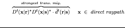
The amplitude
of the transmitted arrival
![]() is
is ![]() , so the strongest
part of the migration image
, so the strongest
part of the migration image
![]() is for
is for
![]() to be along the direct ray shown in Figure a,
which coincides with
the central part of the transmission wavepath
in Figure b.
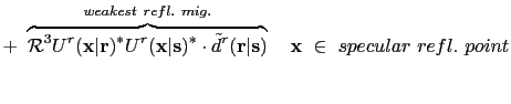
The weakest contribution in
the above approximation is
to be along the direct ray shown in Figure a,
which coincides with
the central part of the transmission wavepath
in Figure b.
The weakest contribution in
the above approximation is
![]() with strength
with strength
![]() ,
and contributes at the specular reflection point shown in
Figure b.
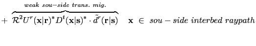
The undesirable contributions
,
and contributes at the specular reflection point shown in
Figure b.
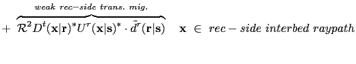
The undesirable contributions![[*]](footnote.png) to the migration image
are along the interbed raypaths with strength
to the migration image
are along the interbed raypaths with strength
![]() shown in Figure c,
which coincide with the central portions of the
rabbit-ear wavepaths in Figure b.
Finally, the most desirable contribution
to the migration image is the Kirchhoff-like image
shown in Figure c,
which coincide with the central portions of the
rabbit-ear wavepaths in Figure b.
Finally, the most desirable contribution
to the migration image is the Kirchhoff-like image
![]() with strength
with strength
![]() . It contributes to the image
at both the specular reflection point in Figure d,
but also to the thick ellipse in Figure b.
. It contributes to the image
at both the specular reflection point in Figure d,
but also to the thick ellipse in Figure b.
For reflection migration, only the Kirchhoff-like term should be used and
contributions from all other terms should be filtered out.
This goal can be accomplished by dip filtering
the Green's functions
to separate upgoing and
downgoing waves, and so
only the Kirchhoff-like kernel
![]() should be used for GDM.
should be used for GDM.
As an example,
the Green's functions associated with the
GDM image
in Figure b can
be filtered to give the separate components in
Figure .
Here, the desirable image is the ellipse in Figure a
(the last term in equation ),
and the undesirable parts are
the smile in Figure b (the 1st term in equation ) and
the rabbit ears in Figures c-d (the 3rd and 4th terms in equation ).
Applying a dip filter to the migration kernels separates the migration image
into the different portions shown in Figures a-d.
Since we are only interested in
imaging the reflector boundary, then only the
migration kernel associated with the ellipse should be used.
|
|
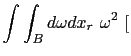
![$\displaystyle \int \int_{B} d \omega dx_r ~ \omega^2~[\tilde d^{t}({\bf {r}}\ve...
...f {r}})]^*~[D^{t}({\bf {x}}\vert{\bf {s}})+ U^{r}({\bf {x}}\vert{\bf {s}})]^* ,$](img61.png)
![$\displaystyle +~ \overbrace{\mathcal RD^{t}({\bf {x}}\vert{\bf {r}})^* D^{t}({\...
...\bf {s}})}^{strong~refl.~mig.}~]
~~~{\bf {x}}~\in~ specular~refl.~pt.+ellipse,$](img68.png)