


Next: Compression of the Migration
Up: Generalized Diffraction-Stack Migration
Previous: Summary
Contents
Computation of the Migration Kernel
The migration kernel in equation ![[*]](crossref.png) can be computed
in one of two ways.
can be computed
in one of two ways.
- Place a source point on the surface at
 , and solve for the field everywhere
in the model
by a finite-difference method to get the Green's function
, and solve for the field everywhere
in the model
by a finite-difference method to get the Green's function
 . Reciprocity says that
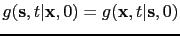 , and if we replace
 then this gives
 .
Thus,
can be convolved with
to give the
migration kernel
.
Thus,
can be convolved with
to give the
migration kernel
 in equation with the receiver at
  and the source at
for all subsurface points
and the source at
for all subsurface points  .
.
- Alternatively, a point source
can be placed at depth
and the field
can be solved everywhere
to get
. This can be cost effective
for target-oriented migration (or waveform inversion)
so that we only
need the Green's functions for point sources along
the boundary
of the target (Dong et al., 2009). Reciprocity says that
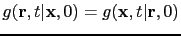 ,
and letting
,
and letting
 yields
.
The migration kernel at
can now be computed by equation . This is the method used by
Liu and Wang (2008) and Dong et al. (2009)
for target-oriented migration.
yields
.
The migration kernel at
can now be computed by equation . This is the method used by
Liu and Wang (2008) and Dong et al. (2009)
for target-oriented migration.
Zhou and Schuster (2002)
demonstrated how to efficiently compute these
migration operators by finite differencing along the leading
portion of the wavefront.
Next: Compression of the Migration
Up: Generalized Diffraction-Stack Migration
Previous: Summary
Contents
Ge Zhan
2013-07-08