Numerical Scheme: Linear Inversion

An alternative to quasi-linear inversion is to invert the given data $\textbf{d}$ by fitting the data with a linear modeling operator $\textbf{L}$ applied to the reflectivity model $\textbf{m}$ . In other words, the problem can be posed as solving the overdetermined system of equations,

$$\textbf{d}=\textbf{Lm}$$ (211)

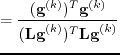
with the iterative solution (Nemeth et al., 1999)

$$\textbf{g}^{(k)} = \textbf{L}^{T}[\textbf{L}(\textbf{m}^{(k)})-\textbf{d}]$$

$$\alpha = \frac{(\textbf{g}^{(k)})^{T}\textbf{g}^{(k)}}{(\textbf{Lg}^{(k)})^{T}\textbf{}\textbf{Lg}^{(k)}}$$

$$\textbf{m}^{(k+1)} = \textbf{m}^{(k)}-\alpha \textbf{g}^{(k)},$$ (212)

where $\alpha$ is the analytical step length and $\textbf{L}^{T}$ is the migration operator. The above calculation of the step length is based on the assumption that the forward modeling and migration operators are exactly adjoint. In practice, it is difficult to achieve exact adjointness, so usually the step length is not accurate. In this case, similar numerical linea search method as in the quasi-linear approach can be used to improve the convergence.