


Next: Forward Modeling of a
Up: Theory
Previous: Theory
Contents
Following Nihei and Li (2006) and Sirgue et al. (2008), the single frequency response of a velocity model
 for a shot at
 can be modelled with the time-domain finite-difference method by solving the equation
![$\displaystyle (\bigtriangledown^{2}-\frac{1}{v^2}\frac{\partial^2}{\partial t^2...
...x},\textbf{s})=-Re[W(\omega_{s})e^{i\omega_{s}t}]\delta(\textbf{x}-\textbf{s}),$](img142.png) |
(35) |
where the source wavelet is a harmonic wave with its amplitude and phase specified by the source
 .
Assuming that the trace length
.
Assuming that the trace length  is long enough to include all the dominant arrivals, the recorded wavefield at the receiver location
 reaches steady state after propagation time
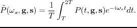
. Therefore, the single frequency response can be extracted with the following formula
reaches steady state after propagation time
. Therefore, the single frequency response can be extracted with the following formula
 |
(36) |
Note that the simulation time is increased from
to  . For a single shot, the above integration can be computed over a single period (
 ) instead of
. Repeating the above solution for different frequencies and digitizing the records give the frequency domain data
) instead of
. Repeating the above solution for different frequencies and digitizing the records give the frequency domain data
 .
.
Next: Forward Modeling of a
Up: Theory
Previous: Theory
Contents
Wei Dai
2013-07-10