


Next: Least-squares Migration
Up: Plane-wave Least-squares Reverse Time
Previous: Introduction
Contents
The theory of least-squares reverse time migration is well established (Symes and Carazzone, 1991; Mulder and Plessix, 2004; Dai et al., 2012).
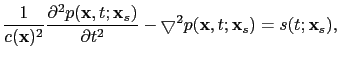
In this section, I will first review the theory of LSRTM assuming the constant density acoustic wave equation,
 |
(14) |
where
 is the velocity distribution, and
 is the pressure field associated with the source term
 . A perturbation in the velocity model
 will generate a wavefield
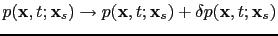 , which obeys the equation
 |
(15) |
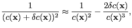
Expanding the velocity term according to
 |
(16) |
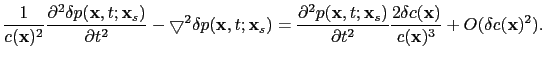
and subtracting equation ![[*]](file:~/utilities/latex2html/icons/crossref.png) from equation yields the wave equation for the wavefield perturbation
from equation yields the wave equation for the wavefield perturbation

 |
(17) |
Neglecting the higher order terms and defining the reflectivity model as
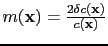 , the above equation becomes
 |
(18) |
Equations and will be used to derive the Born modeling operator. Numerically, the calculation of the reflection data
requires two finite-difference simulations: one to solve equation to obtain the wavefield
, and one to solve equation for the reflection data
. The wavefield
will be recorded at the receiver position
 to give the shot gather
 .
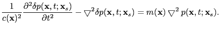
By the adjoint state method (Plessix, 2006), the migration operation of a shot gather
requires two finite-difference simulations, one for the source-side wavefield and one for the receiver-side wavefield:
.
By the adjoint state method (Plessix, 2006), the migration operation of a shot gather
requires two finite-difference simulations, one for the source-side wavefield and one for the receiver-side wavefield:
| |
|
|
(19) |
| |
|
 |
(20) |
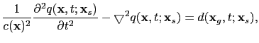
where
 is the receiver-side wavefield.
Note that the source-side wavefield
propagates forward in time but the receiver-side wavefield
propagates backward in time.
The migration image associated with the shot at
is the receiver-side wavefield.
Note that the source-side wavefield
propagates forward in time but the receiver-side wavefield
propagates backward in time.
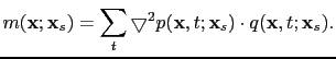
The migration image associated with the shot at
 is produced by applying the imaging condition
 |
(21) |
To simplify the formulas, matrix-vector notation will be used to represent the Born modeling operator
 |
(22) |
where
 is the reflection data vector for the
  shot,
shot,
 is a reflectivity model, and
 represents the Born modeling operator associated with the
shot.
Similarly, the reverse time migration operator can be expressed as
represents the Born modeling operator associated with the
shot.
Similarly, the reverse time migration operator can be expressed as
 |
(23) |
with
 indicating the migration image for the
shot and
indicating the migration image for the
shot and
 representing the migration operator associated with the
shot.
representing the migration operator associated with the
shot.
Subsections
Next: Least-squares Migration
Up: Plane-wave Least-squares Reverse Time
Previous: Introduction
Contents
Wei Dai
2013-07-10